
The Real Estate Game - Part 3
DEBT
In The Complete Guide to Investing in Rental Properties (New York: McGraw-Hill, 2004), I described the use of debt in the following excerpt.
Purchase Price: $500,000
![]() Percent Down: 15.0%
Down
Payment: $75,000
Percent Down: 15.0%
Down
Payment: $75,000
Number Annual Appreciation Rate
of Years 5.0% Ret on Inv 10.0% Ret on Inv 20.0% Ret on Inv
|
1 |
525,000 |
33.3% |
550,000 |
66.7% |
600,000 |
133.3% |
|
2 |
551,250 |
68.3% |
605,000 |
140.0% |
720,000 |
293.3% |
|
3 |
578,813 |
105.1% |
665,500 |
220.7% |
864,000 |
485.3% |
|
4 |
607,753 |
143.7% |
732,050 |
309.4% |
1,036,800 |
715.7% |
|
5 |
638,141 |
184.2% |
805,255 |
407.0% |
1,244,160 |
992.2% |
|
6 |
670,048 |
226.7% |
885,781 |
514.4% |
1,492,992 |
1324.0% |
|
7 |
703,550 |
271.4% |
974,359 |
632.5% |
1,791,590 |
1722.1% |
|
8 |
738,728 |
318.3% |
1,071,794 |
762.4% |
2,149,908 |
2199.9% |
|
9 |
775,664 |
367.6% |
1,178,974 |
905.3% |
2,579,890 |
2773.2% |
|
10 |
814,447 |
419.3% |
1,296,871 |
1062.5% |
3,095,868 |
3461.2% |
|
11 |
855,170 |
473.6% |
1,426,558 |
1235.4% |
3,715,042 |
4286.7% |
|
12 |
897,928 |
530.6% |
1,569,214 |
1425.6% |
4,458,050 |
5277.4% |
|
13 |
942,825 |
590.4% |
1,726,136 |
1634.8% |
5,349,660 |
6466.2% |
|
14 |
989,966 |
653.3% |
1,898,749 |
1865.0% |
6,419,592 |
7892.8% |
|
15 |
1,039,464 |
719.3% |
2,088,624 |
2118.2% |
7,703,511 |
9604.7% |
|
16 |
1,091,437 |
788.6% |
2,297,486 |
2396.6% |
9,244,213 |
11659.0% |
|
17 |
1,146,009 |
861.3% |
2,527,235 |
2703.0% |
11,093,056 |
14124.1% |
|
18 |
1,203,310 |
937.7% |
2,779,959 |
3039.9% |
13,311,667 |
17082.2% |
|
19 |
1,263,475 |
1018.0% |
3,057,955 |
3410.6% |
15,974,000 |
20632.0% |
|
20 |
1,326,649 |
1102.2% |
3,363,750 |
3818.3% |
19,168,800 |
24891.7% |
|
21 |
1,392,981 |
1190.6% |
3,700,125 |
4266.8% |
23,002,560 |
30003.4% |
|
22 |
1,462,630 |
1283.5% |
4,070,137 |
4760.2% |
27,603,072 |
36137.4% |
|
23 |
1,535,762 |
1381.0% |
4,477,151 |
5302.9% |
33,123,686 |
43498.2% |
|
24 |
1,612,550 |
1483.4% |
4,924,866 |
5899.8% |
39,748,424 |
52331.2% |
|
25 |
1,693,177 |
1590.9% |
5,417,353 |
6556.5% |
47,698,108 |
62930.8% |
One additional advantage of using debt is that the interest portion of the payment is tax deductible, because interest is treated as an expense for tax purposes. Since the interest portion of a debt payment is tax deductible, the effective interest rate is lower than it otherwise would be. This provides investors with an added incentive to use debt rather than equity, since they are able to further reduce their cost of funds. Let’s take a moment to look at an example to see how this works.
Loan amount = $100,000
Interest rate = 6.50%
Annual interest paid = $100,000 × 6.50% = $6,500
Investor’s tax rate = 35%
Reduction in taxes = $6,500 × 35% = $2,275
Effective interest rate = ($6,500 − $2,275) = $4,225 ÷ $100,000
= 4.225%
This example assumes a loan amount of $100,000 and cost of funds of 6.50 percent. An investor in a 35 percent tax bracket would realize $2,275 in savings as a result of the reduction in tax liability. The annual cost of funds is reduced from $6,500 to $4,225, which in turn reduces the effective tax rate to 4.225 percent.
EQUITY
Another common method of funding an investment is by raising capital in the form of equity. Whereas debt represents money that is borrowed, equity represents money that is invested. Equity financing can be provided by any number of sources and commonly involves the formation of a legal partnership or corporation. Family, friends, business associates, and private investors can all be good sources of equity financing. One of the main reasons for using equity financing is to minimize the cash flowing out of income- producing properties. The repayment of equity financing can be structured in any number of ways. For example, you can agree with the investor to pay a specified percentage of the profits at the end of each quarter, semiannually, or even annually. You could also agree to defer all payments until such time as the property is sold. Sharing profits with an equity investor can be based on income, capital gains, or any combination of the two. Preserving as much cash as possible, especially in the earlier years of investing when cash reserves tend to be smaller, can mean the difference between success and failure in the real estate business.
Although not as common as lenders who provide financing in the form of loans, or debt, a number of institutional investors are willing to fund investment projects in the form of equity. In other words, instead of lending money to buyers, investors contribute capital in the form of equity. In essence, they become shareholders. Capital contributions from equity investors allow the smaller private investors to leverage up into larger commercial or multifamily properties that they otherwise would not be capable of purchasing.
Equity investors typically require a minimum return on their investment that is higher than if the funds had been borrowed. Furthermore, because they are shareholders, equity investors also expect to share in the profits of a property that result from its sale. Most of the larger institutional investors are looking to place large sums of capital and oftentimes will not even consider a project less than $5 million in size. Since they will fund up to 80 or 90 percent of the capital required, the private investor will need to be prepared to invest a minimum of 10 to 20 percent. Let’s look at an example to see how this might work for a commercial strip center with a purchase price of $5 million.
Purchase price = $5,000,000
Total equity = 20% = $5,000,000 × 20% = $1,000,000
Institutional share = 80% = $1,000,000 × 80% = $800,000
Investor share = 20% = $1,000,000 × 20% = $200,000
Structuring the financing in this manner allows smaller investors the opportunity to acquire larger income-producing properties than would otherwise be possible. In this example, the investor is able to purchase a $5 million commercial property with only $200,000. Instead of the normal 15 to 20 percent down, the investor has to come up with only 4 percent of the total purchase price, as follows:
$200,000
Investor share of total purchase price = —— = 4%
$5,000,000
Institutional firms like partnering with local investors who are familiar with the market in a specific area. Local investors often- times have a good idea of which areas are preferable for various rea- sons. For example, they may have insight into which areas are enjoying positive, even strong, growth and which areas are deteriorating and should likely be avoided. Local investors can also help with, or even be responsible for, the management of the property.
Don’t assume that institutional firms are standing by with an open checkbook waiting to invest in the first property that you bring to them. That isn’t the case. These investors have accumulated large pools of capital because they are very careful, not because they throw money at every opportunity presented to them. As a smaller investor who is familiar with the local market, you will have to carefully select a property that you believe has potential and represents a sound investment. Then you need to be prepared to put together a well-thought-out business plan, which will include data specific to the area and the property, such as the unemployment rate, average vacancy rates, and rental rates for similar properties. Institutional investors are very selective when they purchase properties, so be prepared to sell them not only on the property and the area, but on yourself as well.
PARTNERSHIPS
Combining your own resources with those of a partner is another way to raise financing for investment properties. The type of partner I am referring to in this section is a friend, family member, or business acquaintance. This differs from the large institutional investor described in the previous equity financing section. Partnerships can be structured in a variety of ways. For instance, capital infusions by partners can take the form of debt or equity, partners can play an active or a passive role, and terms for the repayment provisions can be defined in any number of creative ways. While bringing in a partner certainly has its advantages, probably one of the most challenging aspects is finding one you can work with.
If your partner participates simply by loaning money in the form of debt, then a fixed amount will be repaid to that partner under pre- defined terms and conditions. Unlike more traditional sources of debt financing, payments can be structured in any manner the two of you agree on. For example, you may agree to make both principal and interest payments, interest-only payments, or perhaps defer all payments until the property is sold. Regardless of how the payments are structured, the amount repaid is predetermined as set forth in a fully executed promissory note and is not based on the profitability of the property. Furthermore, the two of you may choose to secure the loan by the property, or you may choose to secure it by some other form of collateral, or you may choose not to secure the loan at all. At a minimum, the promissory note should be witnessed and recordable. The two of you may choose not to record the note for any number of reasons, but the partner loaning the money should have the right to record the instrument if he or she so chooses. An alternative to securing debt financing from a partner is to obtain equity financing. If your partner agrees to invest in your project using equity, then he or she will share the risk with you. If your project goes south, your partner’s investment in the project goes south with you. On the other hand, if you hit a home run, your partner will score right along with you. Both you and your partner will enjoy the benefit of sharing in the profits.
Partners may take either an active or passive role in helping you manage and operate the property. For example, you may decide to have your partners actively participate by taking advantage of what- ever skill sets they may have. If they have good management skills, for instance, you may want them to help manage the property. On the other hand, you may choose to have your partners play a completely passive role wherein their only contribution is investment capital. In summary, allowing partners to participate can be beneficial to you by providing additional capital for a project that otherwise may be out of reach financially. Finally, partners may be able to contribute services or specific skills that you may be lacking.
BLENDED FINANCING AND THE WEIGHTED AVERAGE COST OF CAPITAL
When purchasing income-producing properties, especially larger ones, investors often combine several sources of financing, including both debt and equity. For example, an investor may purchase a 450- unit apartment building using a first mortgage for 70 percent of the total purchase price plus improvements, then raising another 15 per- cent of the total purchase price plus improvements through equity arrangements, then borrowing an additional 10 percent of the total for capital improvements from another lender, and finally, investing 5 percent of his or her own capital. Since the four different sources that provide the financing will most likely charge different rates, a blended rate must be calculated. This blended rate is known as the weighted average cost of capital (WACC). A company’s WACC is the average rate of return required by all of its creditors and investors.
Calculating the WACC for a business or company enables its owners to determine the threshold for future projects or investments. If a real estate firm holding a portfolio of properties, for instance, calculated its WACC at 7.40 percent, assuming the firm’s cost of capital was held constant, it would have to be able to earn a minimum of 7.40 percent to justify investing in another property. If the expected return was less than 7.40 percent, the firm would retain its investment resources until a more favorable opportunity presented itself.
An investment firm’s cost of capital is calculated by first deter- mining the weight of each component of debt or equity and then multiplying that weight by its respective cost. Take a moment to study the following formula.
Weighted average cost of capital = (proportion of debt × cost of debt) + (proportion of equity × cost of equity) = WACC
The formula can also be written as follows:
Weighted average cost of capital = (bonds / bonds + securities)
X bond rate + (securities /(bonds + securities) X securities rate = WACC
WACC = (B /B + S) XRb + (S / B+ S) X Rs
where
WACC is the firm’s weighted average cost of capital
B is the value of bonds, or debt, used for financing
S is the value of stocks, or equity, used for financing
RB is the cost of debt, or interest rate
RS is the cost of equity, or the expected return on equity
Now let’s apply the WACC formula to an example. Assume the following:
Value of real estate portfolio = $25 million
Total outstanding debt = $20 million Total outstanding equity = $5 million Average cost of debt = 6.20% Average cost of equity = 10.40%
WACC = ($20,000,000 /$20,000,000 + $5,000,000) X 6.20% + ($5,000,000 / $20,000,000 + $5,000,000) X 10.40% = ($20,000,000//$25,000,000)
X 6.20% + ($5,000,000 / $25,000,000) X 10.40% = (.80 X .0620)
+ (.20 X .1040) = .0496 + .0208 = .0704 = 7.04% = WACC
In this example, the weighted average cost of capital for the real estate portfolio is 7.04 percent. If the investment firm that owned the portfolio decided to purchase another property, its managers would carefully examine the firm’s cost structure. Assuming a similar cost structure was required to purchase the property, then the manager’s threshold would be a minimum of 7.04 percent. That means the total return from the property must yield an income stream of at least 7.04 percent to increase the total return to the firm. Anything less than that means that the cost of financing the property would be greater than the income earned from it and would therefore have a negative impact on earnings.
Although the WACC calculation is a useful tool for individuals or businesses investing on a larger scale, it is just as useful for those individuals or businesses investing on a smaller scale. As an example, an investor buying a $1 million commercial building must pull $200,000 out of her mutual fund, which has been averaging a 12.0 percent rate of return. She will borrow the remaining $800,000 at an interest rate of 6.0 percent. The WACC in this example would be as follows:
WACC = ($800,000 / $800,000 + $200,000) X 12.00% = ($800,000 / $ 1,000,000)
X 6.00% + ($200,000/$1,000,000) x 12.00% = (.80 x .0600) + (.20 x .1200) = .0480 + .0240 = .0720 = 7.20% = WACC
At first glance, it appears that because the WACC is 7.20 percent, our investor is better off leaving her money in the mutual fund so it can continue to earn 12.00 percent rather the 7.20 percent shown in the calculation; however, because financial leverage was introduced, this may or may not be the case. If the property was purchased at a capitalization rate of 8.50 percent, that means its net operating income would be $85,000 annually before interest. Applying a simple interest-only calculation would require annual debt service as follows:
Net operating income = $85,000
Debt service = $800,000 × 6.00% = $48,000
Net income before taxes = $37,000
Now let’s compare the earnings of $37,000 to the yield on our investor’s savings if left in her mutual fund.
Mutual fund savings = $200,000
Expected rate of return = 12.00% Earnings before taxes = $24,000
Difference between investments = $37,000 − $24,000 = $13,000
Yield on investor’s equity = $37,000/$200,000 = 18.50%
In this simple example, by introducing the concept of financial leverage, the investor would be able to earn an 18.50 percent rate of return by purchasing the commercial building versus a 12.00 per- cent rate of return by leaving her money invested in a mutual fund. Calculating the weighted average cost of capital enables the investor to better understand her true cost of capital. Although she is borrowing funds at an interest rate of 6.00 percent, because she is investing funds that would otherwise earn 12.00 percent, her true WACC is 7.20 percent.
OPTIONS
Option agreements are used by investors to gain control of an asset without having to take legal title to it. Options give investors the legal right to purchase an asset at a predetermined price. The use of options is used by investors every day in the stock market to gain control of the rights to either buy or sell various types of securities. An investor could purchase, for instance, a put option for 1,000 shares of Intel with a strike price of $35. This gives the investor the right to sell shares of Intel at $35. The Black-Scholes model is the standard by which options are valued. As with all options, time t is one of the variables that determine its value. Investors have the right to exercise an option at their discretion within a specified period of time. While it is possible that an investor will buy or sell at precisely the right time to lock in a gain, it is also possible that the option will expire worthless and that the investor will lose the money invested to purchase it. In the case of the investor who purchased a put option for 1,000 shares of Intel, it is hoped that the price of the stock will fall so that the investor can sell it at the higher strike price of $35 after having purchased it at any price less than its strike price.
An option works essentially the same way with real estate as it does with a stock. Some sellers may require the purchaser to meet additional obligations, such as assuming responsibility for interest and taxes; however, these items are negotiable. When an option is used with real estate, investors have the legal right to purchase a specified piece of property at a predetermined price within a given time frame. As with stocks, t will eventually expire worthless if the option is not exercised. At some point before the expiration of the option agreement, the investor may exercise her right to purchase the property at whatever price was established. In addition, since a legal interest is held in the property, that interest is usually transferable. This gives the investor the right to sell the property with- out ever taking title to it. Options are a terrific tool investors can use to purchase property with very little cash of their own. This is especially true if another buyer is found before actually having to take title to it. Another benefit of using options is that they provide investors with the ability to limit their risk exposure in a particular property to only the premium paid for the option. If the investor decides not to exercise the right to purchase, the option expires worthless, and only the premium paid for the option is lost. Depending on the value of the subject property, an option may potentially cost tens of thousands of dollars. While this may represent a substantial amount of money, keep in mind that the price paid for an option is relative to the value of the property being sought. Although the Black-Scholes model is the standard used to price options for stocks, option premiums for real estate are typically based on whatever price is negotiated by the parties that have an interest in it. I personally have paid anywhere from about 1 per- cent of the total purchase price to as much as 5 percent for an option.
Some of the real estate investment activities employed by Symphony Homes include the use of options for the development and construction of single-family houses. Options are used to acquire rights to property to build on without ever taking legal title until we are ready to begin construction. The company does, however, have a recordable interest in the property. In Chapter 2, I referred to a recent real estate transaction that was worth $3.3 million. An option agreement was used to acquire the rights to that property, which gives Symphony Homes the ability to build on any one of the lots in an entire community at a predetermined price. When our company has a purchase agreement to build a new home for a client on one of those lots, we then exercise the option on that lot and take legal title to it. Although we do have a pre- determined strike price, or purchase price, on all of the lots, interest and taxes begin accruing from the date the agreement is signed. The advantage to us in this case is that even though we do eventually have to pay those costs, we are able to defer them until we are actually ready to begin construction on a lot. This provision allows us to minimize our outgoing cash flow and thereby retain as much working capital as possible to take advantage of other potential opportunities.
Let’s take a moment to compare the use of an option agreement on this transaction to the use of traditional bank financing. By using an option, we were able to gain control of the lots in an entire community with only 1 percent down. By comparison, purchasing developed land through more traditional means such as bank financing typically requires at least a 20 percent down payment.
Scenario 1: Option Agreement Scenario 2:
Traditional Bank Financing
Purchase price $3,300,000 $3,300,000
Option fee 1% 20%
Total cash required $3,300,000 × 1% = $33,000 $3,300,000 × 20% = $666,000
Difference = $660,000 − $33,000 = $627,000
In this example, using an option agreement allowed me to gain control of an entire community with only $33,000. If I had approached a bank to finance the project, it would have required $660,000 in total cash. Using an option agreement provided me with a net favorable reduction in the amount of cash required of $627,000. I think you would agree with me that this is a significant sum of money. The use of an option here allowed me to take full advantage of the law of leverage by gaining control of real estate valued in excess of $3 million for a meager 1 percent of the purchase price. Now that’s what I call leverage!
The advantages of using an option in this case are twofold. The first advantage is that if we have difficulty selling new homes to prospective buyers in this particular community, we are not stuck with the ongoing burden and cost of owning the lots. The only thing we have at risk is our option money. The second advantage is that if we were to actually purchase the lots, the sale would trigger an increase in taxes due to a new and much higher assessed value, because the value of finished lots is much higher than when the developer first starts improving the land. This is because in the state of Michigan, property values are not reassessed until a transfer of ownership has occurred. They are instead capped at a maximum increase by a change in prices similar to that of the Consumer Price Index (CPI). As the new owners, Symphony Homes would then be obligated to assume the new, higher tax liability.
In summary, the use of options can be an incredibly effective tool for real estate investors who are interested in gaining control of investment property without having to take title to it. Options enable investors to gain control of property with very little money down, which thereby allows them to maximize the use of leverage. I recommend, however, that options agreements be used prudently. Remember that time is one of the variables of an option agreement, and when t expires, so does the option. Carefully study the market as it applies to your particular investment opportunity before commit- ting any capital to it to determine whether the probability of the out- come is favorable. This will help minimize the risk of any loss of capital.
A ratio is a mathematical equation used to express the relationship between sets or groups of numbers. The use of ratios for analyzing income-producing properties is essential to properly and fully understand their respective values. Furthermore, ratios provide a gauge or general rule of thumb so that a specific property’s value can quickly be determined relative to similar properties that may be for sale.
Two precepts must be remembered when applying ratio analysis. The first is the notion that value is relative. Using the logic described here, we have established the precept that indeed, value is relative. This logic leads us to the second precept, which is that performance measurements are relative.
The notion that value is relative leads us to conclude that the performance measurements that capture those values must also be relative. For example, what might be considered a good cap rate in one area might very well be considered poor in another area. These areas do not have to be in different parts of the country, either. They can quite easily be in the same metropolitan area. Since cap rates are a function of property values, and property values are in part determined by the location of the property, an investment property in a less than desirable neighborhood would command a higher cap rate (and lower price) to attract buyers who prefer a higher yield. Conversely, an investment property in a highly desirable neighbor- hood would command a lower cap rate (and higher price) to attract buyers who prefer a higher-quality asset.
The notion that value and performance measurements are relative is essential for investors to both understand and apply. Without this knowledge, it would be very easy to overpay for a property. Be sure to factor these precepts in when analyzing potential investment opportunities.
NET INCOME RETURN ON INVESTMENT
One thing almost all investors have in common is a desire to know the answer to the question, “How much will I make on my investment?” Put another way, investors want to know what the return on their invested dollars will be, or what their return on investment (ROI) will be. The ROI performance measurement can be applied to measure the effectiveness of all types of assets and is especially useful in real estate. The ROI measurement captures the relationship between net income and invested capital, cash flow and invested capital, and the asset’s total return and invested capital.
The first of these measurements, net income return on investment, captures the relationship between net income and invested capital. This is helpful to financial managers who focus primarily on the traditional income statement. Net income is derived by subtracting all items that are classified as expenses for reporting purposes from gross revenues. Net income is calculated both before and after taxes. It gets a little tricky in that whenever a payment is applied to a mortgage, not all of the payment is treated as an expense. For example, the interest, taxes, and insurance portion of a payment are treated as expenses. The principal portion of the payment, however, is treated as a balance sheet item and has no effect on the income statement. When a payment is applied to principal, two things happen. First, cash is reduced, and second, the loan balance is reduced. The balance sheet remains precisely in balance, as one asset is used to reduce a liability by an equivalent amount. The net income ROI performance measurement is calculated as follows:
Net income ROI
gross income − operating expenses − interest − depreciation
= ———————
owner’s equity
CASH RETURN ON INVESTMENT
The second performance measurement is referred to as the cash return on investment, also known as the cash-on-cash return. It is the ratio between the remaining cash after debt service and invested capital, also known as owner’s equity. This ratio differs from the net income ROI in that it excludes all noncash items, such as depreciation expense, and includes the non-income portion of loan payments that are made to principal loan balances. As a general rule, investors tend to focus more on this performance measurement than they do on the net income ROI measurement since it represents the cash return on their investment.
The cash ROI performance measurement is calculated as follows:
remaining cash after debt service
Cash ROI = ————
cash investment
The cash ROI, then, is the ratio between the remaining cash after debt service and invested capital, or owner’s equity. This performance ratio is important to investors because it measures the monthly and annual cash returns on the cash they have invested.
TOTAL RETURN ON INVESTMENT
The third performance measurement is referred to as the total return on investment. The total return on investment is similar to the cash ROI with one important distinction—it accounts for that portion of return that is not cash, namely, the reduction in principal. In other words, it takes into account the portion of the loan that is reduced each period by the payments that are applied to the remaining loan balance, or the principal portion of the loan payment. The total ROI is the ratio between the remaining cash after debt service plus principal payments and invested capital. The total ROI is calculated as follows:
Total ROI
remaining cash after debt service + principal reduction
= ——————
cash investment
The total ROI performance ratio does exactly as its name implies. It provides a measurement of the total return of an investor’s capital by capturing both the cash and noncash portions of the return. The noncash portion is similar to making a house payment amortized over a period of years. The value is there in the form of a buildup of equity and a decrease in the liability, or mortgage, as the loan balance is reduced a little at a time over several years. The gain is realized in the form of cash at the time of sale. The total ROI can be calculated as both before-tax and after-tax performance measurements.
NET OPERATING INCOME
The fourth performance measurement is known as net operating income (NOI). Net operating income is the income that remains after all operating expenses have been paid. It is also the amount of income available to service the property’s debt—in other words, to pay on any outstanding loan balances such as a mortgage or seller- financed note. Net operating income is also the numerator in the quotient used to calculate the capitalization rate. NOI is calculated as follows:
Gross income − total operating expenses = net operating income
The net operating income is a key figure to understand because it is needed to calculate a property’s cap rate. It can also be used to estimate the approximate sales price of an income-producing property. For example, if you know that office buildings in a given market are selling for an estimated cap rate of eight (8 percent), and the NOI from a particular building is $240,000, then the estimated selling price for the building should be approximately $3 million. The calculation is made as follows:
Net operating income
——— = sales price
Cap rate
$240,000
— = $3,000,000
.08
Now take a moment to review Table 6.1. The table provides a detailed example of how NOI is derived in a typical apartment building. These figures will vary widely, of course, among apartment buildings depending on factors such as whether the tenant or the management is paying for utilities, local tax rates, labor costs, and other factors.
Net Operating Income
Operating Revenues Annual
![]() Gross Scheduled Income 700,489
Gross Scheduled Income 700,489
|
Less Vacancy 24,340 |
|
|
Net Rental Income |
676,149 |
|
Utility Income |
71,877 |
|
Other Income—Laundry, Misc. |
16,760 |
|
Gross Income |
764,786 |
|
Operating Expenses |
|
|
General & Administrative |
|
|
Management Fees |
26,767 |
|
Office Supplies |
4,691 |
|
Legal and Accounting |
1,404 |
|
Advertising |
1,938 |
|
Total General & Administrative |
34,801 |
|
Repairs and Maintenance |
|
|
Repairs, Maintenance, Make Readies |
69,664 |
|
Contract Services |
5,088 |
|
Patrol Services |
4,831 |
|
Grounds and Landscaping |
4,751 |
|
Total Repairs and Maintenance |
84,334 |
|
Salaries and Payroll |
|
|
Office |
33,780 |
|
Maintenance |
21,920 |
|
Payroll Taxes |
9,176 |
|
Total Salaries and Payroll |
64,876 |
|
Utilities |
|
|
Electric |
82,459 |
|
Gas |
20,056 |
|
Water and Sewer |
54,548 |
|
Trash |
8,387 |
|
Telephone |
1,378 |
|
Total Utilities |
166,827 |
|
Other |
|
|
Real Estate Taxes |
38,536 |
|
Insurance |
19,447 |
|
Total Other |
57,982 |
|
Total Operating Expenses |
408,821 |
|
Net Operating Income |
355,965 |
CAPITALIZATION RATIO
The fifth performance measurement is referred to as the capitalization ratio, or cap rate, which is the ratio between net operating income and sales price. Like the other performance measurements, the cap rate is a relevant measurement, which means that a favorable cap rate in one market may be considered unfavorable in another market. The cap rate is calculated as follows:
Net operating income
——— = capitalization rate
Sales price
The cap rate is an indicator of value that measures the conversion a single payment or a series of payments, such as in a perpetuity, into a single value. The process of converting income into a single value then is what we refer to as capitalization. The cap rate captures this measurement in a single value. It is very similar to the yield on a financial instrument such as a certificate of deposit. In The Complete Guide to Buying and Selling Apartments (New Jersey: John Wiley & Sons, 2004), I discussed this crucial performance measurement at length. Following is an excerpt from Chapter 4.
As you can see, this ratio is really a very simple calculation used to measure the relationship between the income generated by the property and the price it is being sold for. To help put this in a better perspective for you, let’s refer back to the beginning of this chapter when we discussed certificates of deposits. We knew the value of a CD was calculated by its respective yield. The cap rate measures that exact same relationship!
Present value of CD = income / rate = $10,000/.05 = $200,000
Or to look at it another way . . .
Rate = income / PV = $10,000/ $200,000 = .05 = 5%
Buying an apartment building as related to this equation is really no different than buying a CD from your local bank. As an investor, you are willing to pay or invest a certain amount of capital in order to achieve a desired return. You know that the rates paid by banks for CDs will vary within a given range, let’s say 4%–6%, so you will most likely shop around a little bit to find the most favorable rate. The same is true of apartment complexes. The rate paid, or yield on your investment, will vary within a given range, generally 8%–12%, depending on a variety of market conditions including supply and demand issues, the current interest rate environment, and tax implications imposed by local, state, and federal authorities.
Let’s look at an example. We know that NOI is derived by subtracting total operating expenses from gross income. If you were to pay all cash for an apartment building, then NOI represents the portion of income that is yours to keep (before taxes and capital improvements), or the yield on your investment. If you were considering purchasing an apartment building that yielded $50,000 annually and the seller had an asking price of $800,000, should you buy it? Let’s plug in the numbers to our equation and find out.
Net operating income = $50,000
Sales price = $800,000
Cap rate = NOI / price = $ 50,000 / $ 800,000 = .0625 = 6.25%
In this example, you can see that the asking price of
$800,000 provides us with a yield of only 6.25%.
Let’s assume that comparable properties in this particular market are selling for cap rates of 10%. Armed with that knowledge, we can easily determine a more reasonable value for the property by solving for sales price as follows:
Cap rate = NOI / price
Price = MOI / cap rate = $50,000 / .10 = $500,000
So in this example, based on the limited information we have, we know the apartment is overpriced by $300,000. Understanding this simple, yet powerful equation is fundamental to properly assessing value. Armed with this knowledge, you can quickly determine if the asking price of an apartment building is reasonable.
The cap rate is one of the most important performance measurements available to investors. You can see by the example illustrated here that an investor who is unfamiliar with this key ratio could have potentially overpaid for the apartment building by an astonishing $300,000. I should add that you can’t always rely on the advice or opinion of a real estate agent when it comes to analyzing income- producing properties such as apartment buildings. Many well- meaning agents don’t understand value any better than the average person. Unless agents specialize in multifamily or commercial property, they will most likely not truly understand the value of an income-producing asset. I’ve also met my share of agents who do work in this industry and who still don’t understand value. My advice to you is to familiarize yourself with cap rates by looking at and analyzing as many income-producing properties as you can. By doing so, you will be able to rely on your own judgment and not the opinions of others.
The cap rate is an important performance measurement to be used not only with apartment buildings, but with any kind of income-producing real estate. The cap rate is so important, in fact, that it is the premise on which one of three traditional appraisals methods are based. The income capitalization method, as it is referred to, is discussed in greater detail in Chapter 8, “The Valuation of Real Property.”
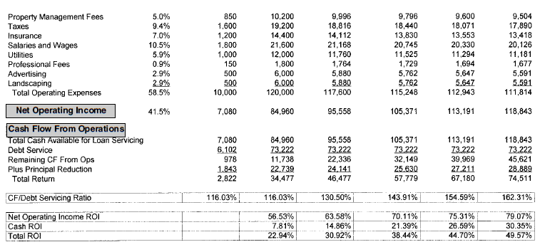
DEBT SERVICE COVERAGE RATIO
The sixth performance measurement is known as the debt service coverage ratio (DSCR). The DSCR is a ratio that measures the relationship between available cash after operating expenses have been paid and the cash required to make the required debt payments. This ratio is especially important to lenders, as they want to ensure that the property being considered for investment purposes will generate enough cash to cover any and all debt obligations. In other words, they want and need to be assured that the real estate is throwing off enough cash to repay the loan. The debt service coverage ratio is calculated as follows:
Debt service coverage ratio = net operating income / principal + interest
= DSCR
The ratio is a simple measure of the relationship of cash generated from an investment to the debt required to pay for that investment. The minimum DSCR varies from lender to lender, but in general it can be as low as 0.75 or as high as 1.40. Most lenders look for a minimum DSCR of 1.00 to 1.20.
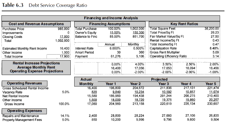
Several factors can impact the DSCR. For example, if an investor increases the amortization period from 20 years to 30 years, the monthly payment will decrease. Since NOI isn’t affected by a change in the amortization period, the DSCR will increase. Take a moment to review Tables 6.2 and 6.3. The two tables are identical except for the amortization period, which is 20 years in
Table 6.2 and 30 years in Table 6.3.
Using a 20-year amortization period in Table 6.2 results in a DSCR of 116.03 percent. If the lender’s minimum required DSCR was 120.00 percent, this property would fail, because it falls below the minimum. That doesn’t necessarily mean the lender would reject the loan, however, as compensating factors may be taken into consideration. Now take a moment to study Table 6.3.
In this example, a 30-year loan amortization period is used, which results in a decrease in the amount of cash required to service the debt each month. The DSCR in this example is 138.65 percent, which compares favorably to the DSCR of 116.03 percent in Table 6.3. Since the lender’s minimum required DSCR is 120.00 percent, the property structured with the longer amortization period of 30 years meets the lender’s minimum requirement.
OPERATING EFFICIENCY RATIO
The next performance measurement is referred to as the operating efficiency ratio (OER). The OER is a computation that measures the operating expenses of an investment property relative to its size. The ratio is useful for both multifamily and commercial real estate properties. It is calculated as the ratio of total operating expenses to total square feet. The result provides a measure of how efficiently the property can be operated. The lower the number, the less it costs to manage and operate the property. The calculation is made as follows:
total operating expenses
Operating efficiency ratio = ——— = OER
square feet
In the examples illustrated in Tables 6.2 and 6.3, the total operating expenses in Year 1 are $120,000 and the total square feet are 38,200. The resulting OER is 3.14, calculated as follows:
$120,000
OER = — = 3.14
38,200
This calculation tells us is that it costs $3.14 per square foot on aver- age to operate the property. The operating efficiency ratio captures
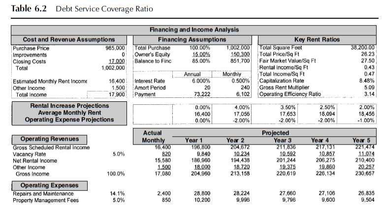
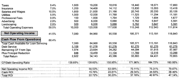
The relationship between operating expenses and size and can there- fore be a useful measurement in evaluating similar properties. If the average OER in a specific market is 3.00, or $3.00 per square foot, then this property would be considered to be within range, but slightly above average.
GROSS RENT MULTIPLIER
The next performance measurement is referred to as the gross rent multiplier (GRM). The gross rent multiplier measures the relation- ship between the total purchase price of a property and its gross scheduled income. It is the ratio of price to income. The GRM calculation is made as follows:
purchase price
Gross rent multiplier = ——— = GRM
gross scheduled income
The GRM is similar to the cap rate in that it captures the relationship between revenues and price; however, there are two primary differences. The first is that while the GRM measures the relationship between gross revenues and price, the cap rate measures the relationship between net revenues, or NOI, and price. The second difference is that one ratio is inverted compared to the other. For example, purchase price is the numerator in the GRM quotient, but it’s the denominator in the cap rate. While a higher cap rate is preferred to a lower cap rate, a lower GRM is preferred to a higher GRM. This is true because the ratio will decrease the lower the purchase price is relative to income. It will also decrease the higher the income is relative to the purchase price.
In the examples illustrated in Tables 6.2 and 6.3, the GRM of 5.09 measures the relationship between the total purchase price and the gross scheduled income in Year 1.
$1,002,000
GRM = —— = 5.09
$196,800
In the model used to make the calculation, both improvements and closing costs have been factored into the analysis. Although there are no improvements in this example, they are typically included if major capital expenditures are expected. If the improvements are expected to increase the gross revenues, that, too, should be taken into consideration. The GRM can be calculated on either an as-is basis with no changes or improvements to the property, or on a pro forma basis, which includes both improvements and the expected increase in revenues that would result from the improvements.
OPERATING RATIO
The next performance measurement used to analyze income producing properties is the operating ratio (OR), which is the ratio between total operating expenses and gross income. Like the operating efficiency ratio, it provides a gauge of how efficiently a given property is being operated. Whereas the OER measures efficiency relative to a property’s total square footage, the OR measures efficiency relative to a property’s income. The calculation is made as follows:
total operating expenses
Operating ratio = ——— = OR
gross income
Depending on the type of income property, an OR can range from about 30 percent to as high as 70 percent or even more. Commercial properties tend to have a lower OR since most of the expenses are passed through to the tenant. Multifamily properties, on the other hand, tend to have a somewhat higher OR since the expenses that are passed through vary. For example, an apartment building being operated as an “all bills paid” property will certainly have higher expenses relative to its income compared to a similar property in which the utilities are paid by the tenants. In the examples illustrated in Tables 6.2 and 6.3, the OR of
58.5 percent measures the relationship between total operating expenses and gross income and is calculated as follows:
$120,000
OR = — = 58.5%
$204,960
The result in this example of 58.5 percent is somewhat on the high side, but does not fall outside the range of normal ratios. An investor looking to create value in an income-producing property would carefully examine each factor that contributes to the operating expenses. In other words, a high OR may signal that repairs and maintenance are abnormally high, or perhaps that management expenses could be trimmed. Conversely, an unusually low OR could signal that not all of the operating expenses are being reported. If repairs and maintenance, for example, are known to average 10 to 15 percent of gross income but are being reported as only 3 or 4 per- cent, then either the property is in exceptionally good condition or not everything is being reported.
BREAK-EVEN RATIO
The final investment performance measure we examine is known as the break-even ratio (BER), which measures the relationship between total cash inflows and total cash outflows. The BER is similar to the OR in that both ratios use total operating expenses as part or all of the numerator and gross income as the denominator. The difference between the two is that the BER includes as part of the numerator the debt service. The BER serves as a performance measurement of cash flows from a property, and the OR serves as a performance measurement of income and expenses.
As the break-even ratio’s name implies, the break-even point is the point at which the total cash inflows are exactly equal to the total cash outflows. A property with a negative cash flow has a ratio greater than 1.0, which means that its cash outflows exceed its cash inflows; conversely, a property with a positive cash flow has a ratio less than 1.0, which means that its cash inflows exceed its cash out- flows. The break-even ratio is calculated as follows:
total operating expenses + debt service
Break-even ratio = ————
gross income
= BER
In the examples illustrated in Tables 6.2 and 6.3, the BER would be calculated by adding the total operating expenses of $120,000 to the debt service of $61,276 and then dividing this sum by the property’s gross income of $204,960. Take a moment to review the calculation.
$120,000 + $61,276
BER = ——— = 88.4%
$204,960
The property in this example has a positive cash flow since the BER is 88.4 percent, which is less than 1.0, or 100 percent. I strongly recommend to investors who have adopted a buy-and-hold strategy to invest in only those properties that have a positive cash flow and a BER of less than 1.0. To do otherwise means that additional cash must be invested each month. A property with a negative cash flow is just like my three growing sons. They are constantly hungry and have to be fed all the time! Unless you have deep pockets, a hungry property will eat your lunch if you’re not careful! If you’re buying a property for the purpose of a quick rehab or flip, then a positive cash flow isn’t as important, because you don’t need as much cash to sustain the project. The negative cash flow, along with the building improvements, is factored into the analysis to determine whether the project represents a viable opportunity.
In summary, each of the 10 real estate investment performance measurements discussed in this chapter can be used by investors to assist in properly analyzing potential investment opportunities. Wise investors who elect to master these principles will no doubt gain greater insight into property values and their worth relative to alter- native opportunities.
In the previous chapter, we examined 10 different real estate investment performance measurements, which enabled us to better under- stand how an income-producing property was performing at a given point in time. These measurements are considered to be static measurements, meaning that they do not take into account a property’s performance over more than one time period. Instead, performance is measured at either a specific point in time or over one period of time, for example, one month or one year. This chapter focuses on advanced methods of real estate investment analysis by measuring performance over multiple periods of time. These financial concepts deal with the time value of money and are especially helpful to individuals investing in real estate over a prolonged period of time.
FUTURE VALUE ANALYSIS
The first of these financial measurements is referred to as future value (FV). The future value concept seeks to determine the value of an investment over multiple periods of time by using the principle of compounding. This principle is used to attribute the interest earned on interest. For example, interest as it applies to money is simply the cost of money to the borrower and the income to the lender. Compound interest is the interest paid on the interest to the borrower and the interest earned on the interest by the lender. The future value concept helps investors to know what a particular property will be worth over a given period of time.
Let’s look at a simple example to better understand the concept of future value and compounding. Banker Smith has offered to pay Investor Jones 5 percent annually for a certificate of deposit held for three years. How much will Investor Jones’s initial investment of $1,000 be worth at the end of the three-year period? To find the solution, we start by introducing the following terms.
PV = present value = the value of an investment today
FV = future value = the value of an investment at some point in the future
i = the interest rate
n = the number of periods
In this example, our terms are applied as follows:
PV = $1,000
FV = ?
i = 5.00%
n = 3 years
FV in Year 1 = $1,000.00 (1 + .05) = $1,000.00 × 1.05 = $1,050.00
FV in Year 2 = $1,050.00 (1 + .05) = $1,050.00 × 1.05 = $1,102.50
FV in Year 3 = $1,102.50 (1 + .05) = $1,102.50 × 1.05 = $1,157.63
In this example, at the end of Year 3, Investor Jones would receive a total of $1,157.63 from Banker Smith. Now let’s look at solving the same problem another way.
FV = PV (1 + i)3
FV = $1,000 (1 + .05)3
FV = $1,000 (1.1576)
FV = $1,157.63
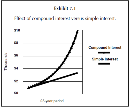
Applying future value principles to real estate helps investors determine the value of their invested capital at some distant point in the future. A working knowledge of the principle of compounding is essential to understanding the effects of returns which are generated over multiple periods of time. It is this compounding component that allows the growth of an investment to accelerate over time. Take a moment to review Exhibit 7.1. Exhibit 7.1 illustrates the difference between growth rates in an initial investment of $1,000 earning 10 percent per year over a 25- year period. The line that curves up sharply is earning interest at a compounded rate, and the line that is linear is earning interest at a simple rate. The future value of a $1,000 investment earning 10 per- cent interest and compounded annually over 25 years is $9,850. By comparison, the future value of a $1,000 investment earning 10 per- cent simple interest annually over 25 years is only $3,400. In this example, the power of compounding has allowed one investment to grow at a rate almost three times faster than the other investment.
Exhibit 7.1
Now take a moment to study Table 7.1. This table provides the factor or value by which an investment can be multiplied to calculate its future value at a specific interest rate and time period. For example, to find out how much a $25,000 investment growing at a rate of 12 percent would be worth in 15 years, locate the corresponding value in the table and multiply it by the amount of the investment, as follows:
FV of $25,000 at 12% in 15 years, where
PV = $25,000
i = 12.00%
n = 15 years
Corresponding value from Table 7.1 = 5.47357
FV = $25,000 × 5.47357 = $136,839
Although Table 7.1 is useful in helping to determine the future value of an investment, it is limited to the rates and time periods within the table. A financial calculator, on the other hand, can be used to calculate the future value of an investment of any size at any rate over any period of time. Most financial calculators are very easy to use. As long as any three of the four variables are known, the fourth one can easily be solved for. As an example, an investor with $5,000 wants to know how long she must hold an investment growing at an annual rate of 8 percent before her investment is worth $25,000. In this example, we must solve for n by entering into the calculator the known values as follows:
PV = $5,000
FV = $25,000
i = 8.00%
Once these values have been entered, then simply solve for n. n = 21 years
In summary, the concept of future value enables businesses and individuals to determine the value of an investment at some point in
Table7.1 Valueof$1atVariousCompoundInterestRatesandTimePeriods
|
Year |
2.00% |
4.00% |
6.00% |
8.00% |
10.00% |
12.00% |
14.00% |
16.00% |
18.00% |
20.00% |
|
1 |
1.02000 |
1.04000 |
1.06000 |
1.08000 |
1.10000 |
1.12000 |
1.14000 |
1.16000 |
1.18000 |
1.20000 |
|
2 |
1.04040 |
1.08160 |
1.12360 |
1.16640 |
1.21000 |
1.25440 |
1.29960 |
1.34560 |
1.39240 |
1.44000 |
|
3 |
1.06121 |
1.12486 |
1.19102 |
1.25971 |
1.33100 |
1.40493 |
1.48154 |
1.56090 |
1.64303 |
1.72800 |
|
4 |
1.08243 |
1.16986 |
1.26248 |
1.36049 |
1.46410 |
1.57352 |
1.68896 |
1.81064 |
1.93878 |
2.07360 |
|
5 |
1.10408 |
1.21665 |
1.33823 |
1.46933 |
1.61051 |
1.76234 |
1.92541 |
2.10034 |
2.28776 |
2.48832 |
|
6 |
1.12616 |
1.26532 |
1.41852 |
1.58687 |
1.77156 |
1.97382 |
2.19497 |
2.43640 |
2.69955 |
2.98598 |
|
7 |
1.14869 |
1.31593 |
1.50363 |
1.71382 |
1.94872 |
2.21068 |
2.50227 |
2.82622 |
3.18547 |
3.58318 |
|
8 |
1.17166 |
1.36857 |
1.59385 |
1.85093 |
2.14359 |
2.47596 |
2.85259 |
3.27841 |
3.75886 |
4.29982 |
|
9 |
1.19509 |
1.42331 |
1.68948 |
1.99900 |
2.35795 |
2.77308 |
3.25195 |
3.80296 |
4.43545 |
5.15978 |
|
10 |
1.21899 |
1.48024 |
1.79085 |
2.15892 |
2.59374 |
3.10585 |
3.70722 |
4.41144 |
5.23384 |
6.19174 |
|
11 |
1.24337 |
1.53945 |
1.89830 |
2.33164 |
2.85312 |
3.47855 |
4.22623 |
5.11726 |
6.17593 |
7.43008 |
|
12 |
1.26824 |
1.60103 |
2.01220 |
2.51817 |
3.13843 |
3.89598 |
4.81790 |
5.93603 |
7.28759 |
8.91610 |
|
13 |
1.29361 |
1.66507 |
2.13293 |
2.71962 |
3.45227 |
4.36349 |
5.49241 |
6.88579 |
8.59936 |
10.69932 |
|
14 |
1.31948 |
1.73168 |
2.26090 |
2.93719 |
3.79750 |
4.88711 |
6.26135 |
7.98752 |
10.14724 |
12.83918 |
|
15 |
1.34587 |
1.80094 |
2.39656 |
3.17217 |
4.17725 |
5.47357 |
7.13794 |
9.26552 |
11.97375 |
15.40702 |
|
16 |
1.37279 |
1.87298 |
2.54035 |
3.42594 |
4.59497 |
6.13039 |
8.13725 |
10.74800 |
14.12902 |
18.48843 |
|
17 |
1.40024 |
1.94790 |
2.69277 |
3.70002 |
5.05447 |
6.86604 |
9.27646 |
12.46768 |
16.67225 |
22.18611 |
|
18 |
1.42825 |
2.02582 |
2.85434 |
3.99602 |
5.55992 |
7.68997 |
10.57517 |
14.46251 |
19.67325 |
26.62333 |
|
19 |
1.45681 |
2.10685 |
3.02560 |
4.31570 |
6.11591 |
8.61276 |
12.05569 |
16.77652 |
23.21444 |
31.94800 |
|
20 |
1.48595 |
2.19112 |
3.20714 |
4.66096 |
6.72750 |
9.64629 |
13.74349 |
19.46076 |
27.39303 |
38.33760 |
|
21 |
1.51567 |
2.27877 |
3.39956 |
5.03383 |
7.40025 |
10.80385 |
15.66758 |
22.57448 |
32.32378 |
46.00512 |
|
22 |
1.54598 |
2.36992 |
3.60354 |
5.43654 |
8.14027 |
12.10031 |
17.86104 |
26.18640 |
38.14206 |
55.20614 |
|
23 |
1.57690 |
2.46472 |
3.81975 |
5.87146 |
8.95430 |
13.55235 |
20.36158 |
30.37622 |
45.00763 |
66.24737 |
|
24 |
1.60844 |
2.56330 |
4.04893 |
6.34118 |
9.84973 |
15.17863 |
23.21221 |
35.23642 |
53.10901 |
79.49685 |
|
25 |
1.64061 |
2.66584 |
4.29187 |
6.84848 |
10.83471 |
17.00006 |
26.46192 |
40.87424 |
62.66863 |
95.39622 |