The Real Estate Game - Part 4

 

 

 

PRESENT VALUE ANALYSIS

 

In the previous section, we examined the concept that deals with the time value of money as it applies to some point in the future. This concept, referred to as future value, allows us to determine the worth of an investment or financial instrument at a future time by introducing the notion of compounding. In this section, we examine the exact opposite concept, known as present value (PV). Present value is derived by adjusting the known future value of an asset at a predetermined interest rate, or discount rate, from a known future point in time backward to its value today. Present value analysis is a tool used by investment professionals every day in a myriad of business decisions, including investing in assets such as equipment to be used for expansion, financial instruments yielding a particular income stream, and income-producing real estate such as office buildings.

 

The notion of present value allows investors to calculate the known future value of an asset or financial instrument in today’s dollars through a process referred to as discounting. For example, it answers a question such as, “How much do I need to invest today if I want to retire in 10 years with $1 million in an investment known to yield 12 percent?” In this example, our terms are applied as follows.

 

PV = ?

FV = $1,000,000

i = 12.00%

n = 10 years

 

To solve this problem, recall the future value equation as follows:

 

FV = PV (1 + i)n

 

Now let’s rewrite the equation to solve for the present value of an asset, as follows:

 

 

FV = PV (1 + i)n

PV = FV 1\(1 + i)n

PV = $1,000,000 1\(1 + .12)10

PV = $1,000,000 1\(3.1058)

PV = $1,000,000 × .321973

PV = $321,973

 

You would need $321,973 to invest today in an asset yielding 12 percent to be able to retire in 10 years with $1 million. By experimenting with the time and interest rate elements of this equation, investors can explore various options that may be available to them. For example, if you don’t have $321,973 today to invest, but you still want to retire with $1 million, you could either extend the value of time or increase the yield. Adjusting either one of these variables would decrease the amount of money needed to achieve your goal.

 

Now take a moment to review Table 7.2. This table provides the factor or value by which an investment can by multiplied to calculate its present value at a specific interest rate and time period. For example, to calculate the present value of an investment discounted at a rate of 12 percent that would be worth $25,000 in 15 years, locate the corresponding value in the table and multiply it by the amount of its future value, as follows:

 

PV of $25,000 at 12% in 15 years, where

FV = $25,000

i = 12.00%

n = 15 years

Corresponding value from Table 7.2 = .18270

PV = $25,000 × .18270 = $4,567

 

The concept of present value calculations is a fundamental and essential tool used by firms in many aspects of operating their businesses. While future value calculations rely on the process of com- pounding to derive value, present value calculations rely on the process of discounting to derive value. Present value calculations allow investors to determine the worth of

an asset whose future

 

Table7.2  PresentValueof$1atVariousCompoundInterestRatesandTimePeriods

 

 

Year	2.00%	4.00%	6.00%	8.00%	10.00%	12.00%	14.00%	16.00%	18.00%	20.00%
1	0.98039	0.96154	0.94340	0.92593	0.90909	0.89286	0.87719	0.86207	0.84746	0.83333
2	0.96117	0.92456	0.89000	0.85734	0.82645	0.79719	0.76947	0.74316	0.71818	0.69444
3	0.94232	0.88900	0.83962	0.79383	0.75131	0.71178	0.67497	0.64066	0.60863	0.57870
4	0.92385	0.85480	0.79209	0.73503	0.68301	0.63552	0.59208	0.55229	0.51579	0.48225
5	0.90573	0.82193	0.74726	0.68058	0.62092	0.56743	0.51937	0.47611	0.43711	0.40188
6	0.88797	0.79031	0.70496	0.63017	0.56447	0.50663	0.45559	0.41044	0.37043	0.33490
7	0.87056	0.75992	0.66506	0.58349	0.51316	0.45235	0.39964	0.35383	0.31393	0.27908
8	0.85349	0.73069	0.62741	0.54027	0.46651	0.40388	0.35056	0.30503	0.26604	0.23257
9	0.83676	0.70259	0.59190	0.50025	0.42410	0.36061	0.30751	0.26295	0.22546	0.19381
10	0.82035	0.67556	0.55839	0.46319	0.38554	0.32197	0.26974	0.22668	0.19106	0.16151
11	0.80426	0.64958	0.52679	0.42888	0.35049	0.28748	0.23662	0.19542	0.16192	0.13459
12	0.78849	0.62460	0.49697	0.39711	0.31863	0.25668	0.20756	0.16846	0.13722	0.11216
13	0.77303	0.60057	0.46884	0.36770	0.28966	0.22917	0.18207	0.14523	0.11629	0.09346
14	0.75788	0.57748	0.44230	0.34046	0.26333	0.20462	0.15971	0.12520	0.09855	0.07789
15	0.74301	0.55526	0.41727	0.31524	0.23939	0.18270	0.14010	0.10793	0.08352	0.06491
16	0.72845	0.53391	0.39365	0.29189	0.21763	0.16312	0.12289	0.09304	0.07078	0.05409
17	0.71416	0.51337	0.37136	0.27027	0.19784	0.14564	0.10780	0.08021	0.05998	0.04507
18	0.70016	0.49363	0.35034	0.25025	0.17986	0.13004	0.09456	0.06914	0.05083	0.03756
19	0.68643	0.47464	0.33051	0.23171	0.16351	0.11611	0.08295	0.05961	0.04308	0.03130
20	0.67297	0.45639	0.31180	0.21455	0.14864	0.10367	0.07276	0.05139	0.03651	0.02608
21	0.65978	0.43883	0.29416	0.19866	0.13513	0.09256	0.06383	0.04430	0.03094	0.02174
22	0.64684	0.42196	0.27751	0.18394	0.12285	0.08264	0.05599	0.03819	0.02622	0.01811
23	0.63416	0.40573	0.26180	0.17032	0.11168	0.07379	0.04911	0.03292	0.02222	0.01509
24	0.62172	0.39012	0.24698	0.15770	0.10153	0.06588	0.04308	0.02838	0.01883	0.01258
25	0.60953	0.37512	0.23300	0.14602	0.09230	0.05882	0.03779	0.02447	0.01596	0.01048

 

 

 

value is known in today’s dollars by discounting it back at a specified or required rate. Understanding the principle of present value enables business owners to make prudent decisions relating to the use of available capital for investment purposes.

 

NET PRESENT VALUE ANALYSIS

 

In the previous section, we learned about using present value formulas to determine the value of an asset in today’s dollars of a known future value at a specific discount rate and period of time. In this section, we examine another financial tool used to measure investments. It’s known as net present value (NPV). The financial analysis of assets using net present value calculations is identical to that of present value calculations with one exception. In a present value calculation, an investor simply wants to determine how much should be invested today to earn a particular rate of return over a given period of time, so solving for PV is all that is required. In a net present value calculation, however, the cost of the investment is already known. Because of this, investors seeking to purchase an income-producing asset use the PV formula to discount the value of the asset back at a predetermined minimum expected rate of return. If the present value of the asset exceeds its cost, the difference is a positive NPV. In this case, the investor would approve the purchase of the asset since it met or exceeded her minimum expected rate of return. If, however, the present value of the asset is less than its cost, the difference results in a negative NPV in which case, the investor would reject the purchase since it did not meet her minimum expected rate of return.

 

Let’s look at an example to better understand how the net present value calculation can be useful to a business. Assume a business that has a minimum required rate of return of 8 percent is considering the purchase of an income-producing asset with a purchase price of

$500,000. The future value of the asset in eight years is expected to be $1.1 million. Using the minimum required rate of return of 8 per- cent, should the company purchase the asset? To answer that question, we must first solve for its present value.

 

PV of $1.1 million at 8% in 10 years, where

FV = $1,100,000

i = 8.00%

n = 10 years

Corresponding value from Table 7.2 = .46319

PV = $1,100,000 × .46319 = $509,512

 

 

To determine the net present value of this investment, the initial cost of the asset must now be subtracted from the present value.

 

NPV = PV − cost

NPV = $509,512 − $500,000 = $9,512

NPV = $9,512

 

Since the NPV is positive, it meets the minimum rate of return required by the business and therefore merits further consideration. A NPV greater than zero means that not only does the asset meet the minimum rate of return, but by definition, it actually exceeds it. By substituting the actual cost of the asset for PV, we can solve for i using a financial calculator, as follows:

 

PV = $500,000

FV = $1,100,000

n = 10 years

i = ?

 

Using a financial calculator, enter the values as illustrated for each of the three known variables. Be sure to enter the PV of $500,000 as a negative value since it represents a cash flow out. All other variables should be entered as positive values. The solution for i is as follows:

 

PV = $500,000

FV = $1,100,000

n = 10 years

i = 8.20%

 

 

 

To summarize, the yield on this investment is 8.20 percent, which exceeds the minimum rate of return required by the business. When analyzing these types of investment opportunities, recall that firms must take into consideration their cost of capital. In this example, if the company’s cost of capital was 6.00 percent, investing in the asset would yield an incremental 2.20 percent. The net present value calculation is a tool commonly used by investors from many different industries, including real estate.

 

INTERNAL RATE OF RETURN

 

In the previous section, the financial analysis principle of net present value enabled us to first calculate the present value of an investment and then subtract the actual cost of the asset from its present value. The NPV calculations were made with a minimum rate of return already established by the firm. In this section, in- stead of solving for the NPV, we solve for the internal rate of return (IRR). The IRR calculation measures the yield or rate of return on an investment rather than its present value. The present value is assumed to be the initial cost of the asset. The IRR calculation measures the yield from a series of cash flows across a specified period of time and includes the cost of the asset, the cash flows from the asset, and the salvage value of the asset at the end of its useful life. In the case of plant and equipment, an asset’s useful life may be exhausted at the end of a period due to functional or technical obsolescence. The useful life of real estate, which may actually increase in value over time, is said to be exhausted when the property is divested.

 

Let’s look at an example. Assume Investor Lincoln wants to add an additional space to a small retail strip center. Construction costs to add the space are estimated to be $100,000. As illustrated in Table 7.3, Lincoln has two choices. In Scenario 1, he can lease the space to Tenant A on a lease-option agreement for three years at a rate of $10,000 per year and then sell the space at the end of the three-year period for $110,000. In Scenario 2, he can lease the space to Tenant B on a lease option agreement for six years at a rate of $10,000 per year for the first three years and $12,500 for the next three years, then sell the space at the end of the six-year period for $120,000.

 

The internal rate of return in Scenario 1 is 12.94 percent. The income generated from three years’ worth of cash flows is the equivalent of earning an annualized rate of return of 12.94 percent on Investor Lincoln’s initial investment of $100,000. If, however, Investor Lincoln chooses to hold the property for six years, his yield increases to 13.40 percent. Because the IRRs in this example are marginally close, there may be other factors such as tax issues that could affect Lincoln’s decision to choose one scenario over the other; however, with all other things being equal, the higher yield in Scenario 2 suggests that Investor Lincoln should choose this alter- native over Scenario 1.

 

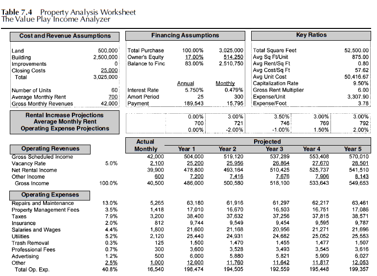
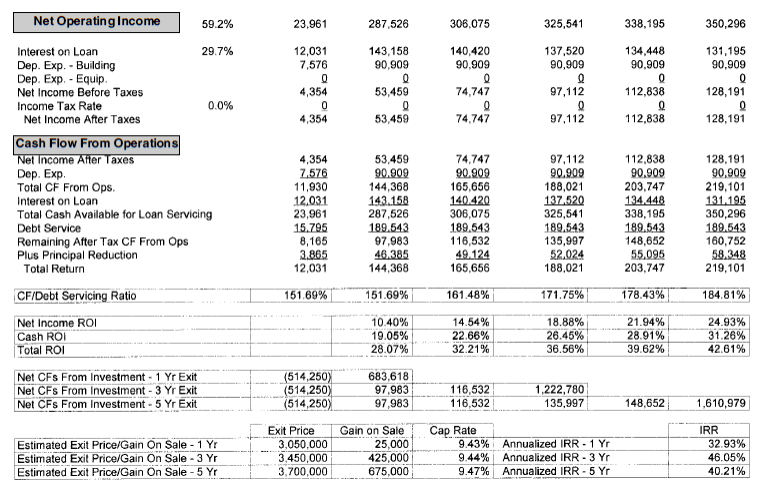
Let’s look at another example using The Value Play Income Analyzer, a proprietary model used for analyzing income properties such as apartment buildings. In Table 7.4, the cash flows of a 50-unit apartment building are examined to determine its respective internal rate of return.

 

In Table 7.4, note the net cash flows from investment section in the lower portion of the table. This section is used to display the net cash flows from the property. The first value in the Year 1 exit section of −$514,250 is a cash-flow-out value that represents the owner’s initial equity. This is followed by a cash-flow-in value of

$683,618, derived by adding the following values.

 

 

Table 7.3   Internal Rate of Return

 

Cash Flows  Scenario 1  Scenario 2

 

Initial Investment      (100,000)   (100,000)

Cash Flow in Year 1     10,000      10,000

Cash Flow in Year 2     10,000      10,000

Cash Flow in Year 3     120,000     10,000

Cash Flow in Year 4                 12,500

Cash Flow in Year 5                 12,500

Cash Flow in Year 6                 132,500

Internal Rate of Return 12.94%      13.40%

 

 

 

Owner’s equity    $514,250

After-tax cash flows    $97,983

Principal reduction     $46,385

Gain on sale      $25,000

Total $683,618

 

The cash flow in value of $683,618 assumes the owner sells the property at the end of Year 1 at a cap rate of 9.43 percent, which is comparable to the 9.50 cap rate at the time of purchase (shown in the key ratios section). If the property was sold at the end of the first year, based on its projected cash flows it would earn an internal rate of return of 32.93 percent. Take a moment to review the net cash flows from investment in Year 3. The initial cash flow out, which is the owner’s equity, of $514,250 is the same as in the Year 1 scenario. The income earned from Years 1, 2, and 3 is then factored in, as well as the reduction in principal and gain on sale of $450,000. Based on the projected cash flows in the Year 3 scenario, the property would generate an IRR of 46.05 percent. Now take a moment to examine the net cash flows from investment in Year 5. The cash flows are derived in the same manner as in the previous two scenarios, but include income and principal reduction for Years 4 and 5 as well. Based on the projected cash flows in the Year 5 scenario, the property would earn an internal rate of return of 40.21 percent.

 

While the internal rate of return calculation is widely used by investors to measure the yield on a series of cash flows, there is one caveat. The IRR calculation works best when the initial cash flow is negative and all subsequent cash flows are positive. Additional  negative  values  in  the  cash  flow  stream  can  potentially create multiple solutions. In an excerpt taken from Investment Analysis for Real Estate Decisions  (Chicago: Dearborn Trade, 1997, p. 222), authors Greer and Kolbe note that the IRR calculation can be problematic under certain conditions. The authors assert the following.

 

 

 

 

 

 

 

 

 

 

 

 

Mathematicians and analysts alike have attempted to resolve the problems that occur with IRR calculations resulting from the reversal in signals in a series of cash flows. Three of the more common methods used to address these issues are (1) the modified internal rate of return, or MIRR, (2) the adjusted rate of return, and (3) the financial management rate of return. According to Greer and Kolbe, the MIRR method “solves the multiple root problem by discounting all negative cash flows back to the time at which the investment is acquired and compounding all positive cash flows forward to the end of the final year of the holding period.” The modified approach eliminates the reversal-of-signals problem and provides a unique solution for a series of cash flows. The adjusted rate of return method assumes the investor has in essence borrowed funds from one period and repaid them in another period, again attempting to deal with positive and negative changes in values. Finally, the financial management rate of return method, developed by M. Chapman Findley and Stephen D. Messner, integrates two intermediate rates. The first, a cost-of-capital rate, is applied to negative that which are discounted back to the beginning of the investment time period where t = 0. The second rate is a reinvestment rate and is applied to positive values that are compounded forward to the end of the investment time period.

 

 

PROPERTY MANAGEMENT vs ASSET MANAGEMENT

 

Property management as the name indicates is the management of an the property asset of another. Typically when more than one property is involved a further abstraction of management of the property portfolio is performed by an asset manager who is tasked with managing the performance of multiple properties for an ownership interested party. A property manager manages and maintaines one or more properties on a day to day basis from a down up approach and asset manager has a top down performance perspective. A manager may report a high turnover due to obselecence of a subject properties features. An asset manager, upon learning these facts notifies the owner and may be authorizes to move profits from another portfolio property to another to improve the overall profitability to the portfolio holder.

 

In summary, this chapter has focused on several advanced methods of real estate investment analysis by measuring performance over multiple periods of time. These financial analysis tools enable individuals and businesses to evaluate investments extending over various periods of time and having various streams of cash flow. Most financial analysis methods use discounting and compounding calculations to express the sum of a stream of cash flows in either present value or future value terms, thereby enabling investors to make decisions based on predetermined minimum rates of return.

 

The Valuation of Real Property

 

APPRAISAL DEFINED

 

n appraisal is an estimate of an object’s worth or value. Appraisals are used to determine the value of both personal property and real property. For example, you may want to have an independent appraisal done on a diamond ring with a $20,000 price tag before investing that kind of money in it. The appraisal could then be used for insurance purposes in the event the ring was lost or stolen. Appraisals are also used to determine the worth and value of real property, such as land or buildings. In Income Property Valuation (Massachusetts: Heath Lexington Books, 1971, p. 9), author William N. Kinnard states the following as it relates to the appraisal process:

 

An appraisal is a professionally derived conclusion about the present worth or value of specified rights or interests in a particular parcel of real estate under stipulated market conditions or decision standards. Moreover, it is (or should be) based on the professional judgment and skill of a trained practitioner. Its conclusions should be presented in a thoroughly logical and convincing way to a client or an interested third party who requires the value estimate to help make a decision or solve a problem involving the real estate in question.

 

An appraisal opinion is usually delivered in written form. A professional appraisal report should contain as a minimum the essential ingredients of an appraisal identified as (1) the identity and legal description of the real estate; (2) the type of value being estimated; (3) the interests being appraised; (4) the market conditions or decision standards in terms of which the value estimate is made (frequently identified by specifying an “as of” date or effective date for the appraisal); and (5) the value estimate itself. Moreover, the report should indicate the data and reasoning employed by the appraiser in reaching his value conclusion, any special or limiting conditions that impinged on his analysis and conclusion, and the appraiser’s certification and signature.

 

THE NATURE OF PRICE AND VALUE

 

As Kinnard clearly states, the process for appraising real property is well defined and specific. Although objective in its format, property values vary widely for many reasons. A 1,000-square-foot house with three bedrooms and two baths, for example, may be worth only $60,000 in Dallas, Texas, while in Hollywood, California, that same house may sell for $150,000. Real estate values are impacted by many different micro- and macroeconomic forces, including supply and demand issues, the current interest rate environment, local and national economic conditions, the desirability of the location, and differences in tax rates. The same appraisal standards applied to a particular piece of real property in one region may yield entirely different results for a similar piece of real property in another region. Likewise, an appraisal of those same properties today would almost certainly be different than an appraisal conducted 10 years ago.

 

Although the terms price and value are similar in meaning, they are not the same. An appraisal is an estimate of value and provides no indication of what price will actually be paid for a piece of real property. For example, an individual shopping for a new refrigerator will first determine all the desired features she must have, and then begin to shop for one matching her requirements. Once a model is selected, she will then most likely shop around at several locations to determine which store is offering the best price. By purchasing the refrigerator at the lowest price available, not only is the buyer able to save money, but she is also said to have received the best value. Although two identical refrigerators at two different locations may have the same resell value, the one that originally sold for less money has a greater equivalent value.

 

The appraisal provides the basis for price, but buyers and sellers are free to negotiate. Kinard asserts, “In the perfect market of economic theory, informed and rational buyers would pay no more, and informed and rational sellers would accept no less, than the present worth of the anticipated future benefits from ownership of an asset.” As a result of various differences in economic conditions, however, the actual price paid may be, and often is, different than the stated value in an appraisal report. Price is therefore a reflection of the past. It is what has already occurred. Value, on the other hand, reflects the price that should be paid “in the perfect market of economic theory.” Value is therefore a forecast of price. It is what may occur at some point in the future, not what has occurred at some point in the past.

 

 

 

THREE PRIMARY APPRAISAL METHODS

 

Three primary methods are used by appraisers to determine the value of real estate: the replacement cost method, the sales comparison method, and the income capitalization method. Each method of valuation has its place and serves a unique function in assessing the worth of real property. Commercial properties such as retail centers, office buildings, and apartment complexes, for example, rely primarily on the income method, while single-family houses typically rely on the sales comparison method.

 

REPLACEMENT COST METHOD

 

The replacement cost method, or cost approach, is most commonly used for estimating the replacement value of physical assets for

 

Three primary appraisal methods.

 

1. Replacement cost method

2. Sales comparison method

3. Income capitalization method

 

insurance purposes. For example, should a house be destroyed in a hurricane, an insurance company would want to know the actual cost to replace it. The income method and the sales comparison method are of little or no consequence in estimating replacement costs. The insurance policy you have on your personal residence most likely includes a replacement cost policy with built-in premium adjustments that automatically increase each year due to rises in labor and material costs. Butler Burgher, Inc., an appraisal firm in Houston, Texas, stated the following in an appraisal report that was completed for one of my apartment projects.

 

The cost approach is based on the premise that the value of a property can be indicated by the current cost to construct a reproduction or replacement for the improvements minus the amount of depreciation evident in the structures from all causes plus the value of the land and entrepreneurial profit. This approach to value is particularly useful for appraising new or nearly new improvements.

 

The replacement cost approach is most commonly used when estimating the actual costs associated with replacing the physical assets of a house or building. For example, for an office building completely destroyed by fire, the value established from the cost approach would be useful in helping to determine exactly how much an insurance company would pay for the resulting damages.

 

An additional factor taken into consideration when the replacement cost approach is used is depreciation, which encompasses deterioration, functional obsolescence, and external obsolescence. Deterioration is said to occur when property loses value because of average wear and tear over a period of time. For example, a 10- year-old roof that has a 25-year life is said to have deteriorated, or depreciated, by 10/25, or 40 percent. Functional obsolescence is described as a loss in property value resulting from outdated home designs or mechanical equipment. The value of a house with only gas space heaters rather than central heating, for example, would be adversely affected. Finally, external obsolescence is described as a loss in property value resulting from changes in the surrounding neighborhood or community. For instance, the value of a house would be adversely affected if it were located in a neighborhood that had experienced a significant increase in crime. An increase in traffic and noise levels may also contribute to a decline in value.

 

The underlying rationale of the replacement cost approach is that an informed buyer would not be willing to pay more for a particular house than the cost of building an identical house on a comparably sized lot in a similar neighborhood. The basic formula for calculating the replacement cost approach is as follows:

 

Replacement cost = cost of construction − depreciation

+ land value

 

Let’s look at an example. Assume the subject property is similar in design, size, and quality to a new house that costs $100,000 to build, not including the lot. The subject property is 30 years old and has depreciated in value by 25 percent due to normal wear and tear, as well as a general decline in the neighborhood in which it is located. The value of the lot is estimated at $20,000. Using the replacement cost approach, the value of the subject property is calculated as follows:

 

 

Replacement cost = $100,000 − ($100,000 × 25%) + $20,000

 

Replacement cost = $100,000 − $25,000 + $20,000 = $95,000

 

In this example, since the subject property has declined in value, using the replacement cost approach indicates a value of $95,000. This compares to a total value of $120,000 for a new house, which includes a comparable lot, for a difference of $25,000, the amount of loss suffered by the subject property from depreciation.

 

SALES COMPARISON METHOD

 

The second primary appraisal method is the sales comparison method, or market approach, which is the method deemed most appropriate for the proper determination of value for single-family houses. This includes both owner-occupied and non-owner- occupied single-family dwellings. The sales comparison method is by far the most commonly used approach of the three methods, because the number of single-family dwellings is much greater than any other type of property. This method is based on the logic that the price paid for recent sales of like properties represents the price buyers are willing to pay and is therefore representative of true market value. The price paid may vary for many reasons, including changes in interest rates, changes in unemployment rates, changes in general economic conditions, as well as changes in the cost of materials and land. All of these factors combine to cause changes in the supply and demand of available properties.

The sales comparison method is based on the premise of substitution and maintains that a buyer would not pay more for real property than the cost of purchasing an equally desirable substitute in its respective market. This method also assumes that all comparable sales used in the appraisal process are legitimate arm’s-length trans- actions to help ensure accuracy of the data used in the report. The sales comparison method furthermore provides that comparable sales used have occurred under normal market conditions. For example, this assumption would exclude properties bought and sold under  foreclosure  conditions—that  is,  those  purchased  from  a bank’s real estate owned, or REO, portfolio.

 

The sales comparison method typically examines three or more like properties and adjusts their value based on similarities and differences among them. For example, if the subject property had a two-car garage and the comparable property had a three-car garage, an adjustment would be made for the difference to bring the values more in line with each other. In this case, the comparable property’s value would be adjusted downward to compensate for the additional garage unit. In other words, the value of the additional garage unit is subtracted to make it the equivalent of a two-car garage. Butler Burgher provides further clarification of the sales comparison method:

 

The sales comparison approach is founded upon the principle of substitution which holds that the cost to acquire an equally desirable substitute property without undue delay ordinarily sets the upper limit of value. At any given time, prices paid for comparable properties are construed by many to reflect the value of the property appraised. The validity of a value indication derived by this approach is heavily dependent upon the availability of data on recent sales of properties similar in location, size, and utility to the appraised property.

 

The sales comparison approach is premised upon the principle of substitution—a valuation principle that states that a prudent purchaser would pay no more for real property than the cost of acquiring an equally desirable substitute on the open market. The principle of substitution presumes that the purchasers will consider the alternatives available to them, that they will act rationally or prudently on the basis of their information about those alternatives, and that time is not a significant factor. Substitution may assume the form of the purchase of an existing property with the same utility, or of acquiring an investment which will  produce an income stream of the same size with the same risk as that involved in the property in question. . . .

 

The actions of typical buyers and sellers are reflected in the comparison approach.

 

According to Butler Burgher, the sales comparison appraisal method examines like properties and adjusts their respective values based on similarities and differences between them. This method is most often used in valuing single-family houses. Recall that the objective of using this method is to determine the subject property’s value. Unlike the cost approach, which seeks to establish the cost of reconstruction for the subject property, the sales comparison approach seeks to establish its market value. Recall also that the market value of a property is not the same as its price. The appraiser’s objective is to determine a value that reflects the most likely price a buyer is willing to pay for a particular property given similar properties to choose from.

 

While the use of sales comparables, or comps, as they are also referred to, is an important factor to consider in the analysis of estimating the value of larger income-producing properties, greater weight is usually given to the income capitalization method dis- cussed in the next segment. The sales comparison method is designed to examine and compare the physical attributes of real property, not the income generated by it.

 

INCOME CAPITALIZATION METHOD

 

The third primary appraisal method is the income capitalization method, used to value real property that generates some type of income, which is employed for investment purposes. In Income Property Valuation, author Kinard describes the process of capitalization as follows:

 

Real estate is a capital good. This means that the benefits from owning it—whether in the form of money income or amenities, or both—are received over a prolonged period of time. Operationally, this means more than one year; in fact, it is typically for 10, 20, 40 or more years.

 

In all economic and investment analysis, of which real estate appraisal is an integral part, the value of a capital good is established and measured by calculating the present worth, as of a particular valuation date, of the anticipated future benefits (income) to the owner over a specified time period. The process of converting an income stream into a single value is known as capitalization. The result of the capitalization process is a present worth estimate. This is the amount of capital that a prudent, typically informed purchaser- investor would pay as of the valuation date for the right to receive the forecast net income over the period specified.

 

Kinard’s succinct description of capitalizing an asset clarifies the process and is so profound that it bears repeating: “The process of converting an income stream into a single value is known as capitalization.” The income capitalization method, then, is appropriately used to value buildings like retail centers, office buildings, mini storage units, industrial buildings, mobile home parks, and multifamily apartment buildings, to name a few. The capitalized value from income-producing real estate is derived directly from the net cash flow or income generated by the asset. Investors compare the rates of return produced from various types of assets against their perceived risks and invest their capital accordingly. Assuming that risk is held constant, an investor’s return on capital is the same regardless of whether it is derived from real estate, stocks, or bonds. To more fully understand the income capitalization method, let’s turn once again to Butler Burgher.

 

The income capitalization approach is based on the principle of anticipation which recognizes the present value of the future income benefits to be derived from ownership of real property. The income approach is most applicable to properties that are considered for investment purposes, and is considered very reliable when adequate income/ expense data are available. Since income producing real estate is most often purchased by investors, this approach is valid and is generally considered the most applicable.

The income capitalization approach is a process of estimating the value of real property based upon the principle that value is directly related to the present value of all future net income attributable to the property. The value of the real property is therefore derived by capitalizing net income either by direct capitalization or a discounted cash flow analysis. Regardless of the capitalization technique employed, one must attempt to estimate a reasonable net operating income based upon the best available market data. The derivation of this estimate requires the appraiser to 1) project potential gross income (PGI) based upon an analysis of the subject rent roll and a comparison of the subject to competing properties, 2) project income loss from vacancy and collections based on the subject’s occupancy history and upon supply and demand relationships in  the  subject’s  market ...,  3)  derive  effective gross income (EGI) by subtracting the vacancy and collection income loss from PGI, 4) project the operating expenses associated with the production of the income stream by analysis of the subject’s operating history and comparison of  the subject to  similar  competing properties, and 5) derive net operating income (NOI) by subtracting the operating expenses from EGI.

 

To summarize Butler Burgher’s remarks, the present value of a capital asset is directly related to its future net operating income. To more fully understand the income capitalization method, let’s break it down to its most basic level by analyzing a simple financial instrument such as a certificate of deposit, or CD. When people buy CDs, they invest a specified dollar amount that earns a predetermined rate of interest for a predetermined period of time. Let’s look at a simple example. Assuming a market interest rate of 4.0 percent, how much would an investor be willing to pay for an annuity yielding $4,000 per annum? The answer is easily solved by taking a ratio of the two values, as follows:

Present value = income / rate = $4,000 / .04 = $100,000

 

In other words, if an investor purchased a certificate of deposit for $100,000 that yielded 4.0 percent annually, she could expect to earn $4,000 over the course of a one-year period. It doesn’t matter whether the income continues indefinitely. The present value, or capitalized value, remains the same and will produce an income stream of $4,000 as long as she continues to hold the $100,000 certificate of deposit. In this example, we have converted the income stream of $4,000 into a single value, which is $100,000. The process for estimating multifamily and commercial properties is essentially the same. The expected future income stream is converted into a single capital value. Let’s take a moment to compare the formula for calculating the present value of a CD to the formula for calculating the present value, or capitalized value, of an income-producing property such as an apartment building.

 

 

Present value of CD = income / rate = 4,000 / .04 = $100,000

 

 

Present value of apartment building

= net operating income / capitalization rate = $4,000 / .08 = $50,000

= net operating income / price = $4,000 / $50,000 = 8.0%

 

Can you see how similar these formulas are? In principle, they are identical. In this example, an individual who invests $100,000 in a certificate of deposit with a yield of 4.0 percent will earn an income of $4,000. Since the yield on the apartment building is higher at 8.0 percent, only $50,000 is needed to earn an income of $4,000. In both examples, the income stream produced by the two assets is converted into a single capital value. The process is very much the same for determining the value of a company’s stock. The ratio is referred to as a P/E ratio. It is the ratio of the price of a given company’s share of stock to the earnings generated by that company, as follows:

 

 

P/E ratio = price/ earnings = $10.00 / $1.00 = 10

 

 

 

Inverse of P/E ratio = E/P ratio = earnings / price = $1.00 / $10.00 = 10

 

 

Present value of stock = income / rate = $1.00 / .10 = $10.00

 

In this example, an investor purchasing one share of stock for a price of $10.00 could expect to earn a 10 percent return, or $1.00. Whether you are attempting to estimate the value of a certificate of deposit, an income-producing property, or a share of stock, the process is the same. The income stream from each asset is converted into a single capital value. The yield on each asset is different, how- ever, as a result of various risk premiums assigned by their respective markets. The certificate of deposit is essentially a risk-free investment with a guaranteed rate of return and therefore offers the lowest yield. The apartment building carries more risk due to the dynamics of the both micro- and macroeconomics, which affects housing and therefore offers a somewhat higher yield. Finally, the share of company stock carries even greater risk due to the volatility inherent in the stock market, measured as beta, and therefore offers the highest yield among the three asset classes.

 

In summary, each of the three primary appraisal methods serves a unique function by estimating value using different approaches. Depending on the type of property being appraised, all three approaches may be taken into consideration, each with its respective weight applied as deemed appropriate. Butler Burgher asserts, “The appraisal process is concluded by a reconciliation of the approaches. This aspect of the process gives consideration to the type and reliability of market data used, the applicability of each approach to the type of property appraised and the type of value sought.”

 

Financial statements are crucial to those who use them by providing information necessary to make decisions regarding an organization. Users of financial statements are classified as either internal or external. Internal users of financial statements include accounting and finance groups, managers, senior executives, and board members. This group uses statements to measure the progress of the company, to evaluate its strength, and to identify areas where improvement is needed. External users of financial statements typically fall into one of three categories: investors, the government, and the general public. Investors include both creditors and debtors, who rely on information from financial statements to make funding decisions regarding equity and debt. Government agencies include local, state, and federal tax authorities, as well as various regulatory agencies. Finally, for corporations that are publicly traded, information is provided to the general public.

 

Financial statements represent the end product of the accounting process. For example, all of the information contained on an income statement is the end result of hundreds or even thousands of individual inputs. The information presented on the report is the end result of those individual inputs. Every time inventory is purchased and later resold, an entry must be made in the accounting system. Inventory becomes a cost of goods sold and flows through the system as an expense; when the item is sold, that sale is treated as revenue. The difference between revenue and cost of goods sold is income. When operating an income-producing property, services, not inventory, generate the revenue, and items such as administrative costs, employees, interest, and taxes are treated as expenses. The difference between the revenue and the expenses is income.

 

When setting up an accounting system, there are several things to consider. For example, a business must determine whether it will operate on an accrual system of accounting or on a cash system. Under the accrual method of accounting, revenue is recognized when goods and services are rendered, not when cash is received. For example, if the owner of a commercial office building operating under the accrual method purchased a one-year insurance policy in June, she would record each month the expense associated with the portion of the premium that had been used. When the policy is initially purchased, rather than recording it as an expense, it is recorded as an asset, typically under the category of prepaid insurance. With each passing month, one-twelfth of the premium is removed from the prepaid insurance and treated as an expense. The accrual method of accounting attempts to more closely match both revenues and expenses with the period in which they occur rather than when cash is exchanged. This method is said to have a smoothing effect on a company’s income statement. Almost all larger businesses use the accrual method of accounting, and many smaller business do as well.

 

The cash method of accounting, on the other hand, recognizes both revenues and expenses at the time payment is made. If, for example, the owner of several rental houses purchased individual insurance policies at various times throughout a given period and expensed the entire amount at the time the policies were paid for, he would be using the cash method of accounting. The cash method of accounting matches both revenues and expenses with the period in which cash is exchanged rather than with the period in which they occur. Although some smaller businesses use the cash method of accounting, very few, if any, larger businesses use this method.

 

All standards of accounting are governed by what are called generally accepted accounting principles (GAAP). Financial accounting and reporting assumptions, standards, and practices that an individual business uses in preparing its statements are all regulated by GAAP. The standards for GAAP are prescribed by authoritative bodies such as the Financial Accounting Standards Board (FASB). The FASB is an independent, nongovernmental body which consists of seven members. The standards applied by FASB are based on practical and theoretical considerations that have evolved over a number of years in reaction to changes in the economic environment. Rulings issued by the board are recognized as being authoritative.

 

The three common financial statements most useful for income- producing properties are the income statement, balance statement, and cash flow statement. These statements are used to report the financial condition of a company on a periodic basis, such as monthly, quarterly, or annually. A prospective purchaser of an income-producing property would be classified as an external user of these financial statements. In order to properly and accurately assess the financial condition of this type of property, the broker or seller should furnish the prospective buyer with the most recent two or three years of historical operating statements. The ability to review several periods provides investors with a more complete picture of the property’s capacity to perform over an extended period of time. Investors should be able to detect any trends that are present, such as the regular increase of rents. Conversely, an investor who observed flat or declining rents with corresponding increases in the vacancies would possibly conclude the market in that particular area has softened. This could also indicate management problems, which can be much more easily overcome than a deteriorating market.

 

Historical operating statements are not always readily available for one reason or another, and when they are, they are not always accurate, especially on smaller properties where no formal accounting system is used. Sellers or their brokers should be able to provide a minimum of the most recent 12-month period of operating data. The trailing 12-month period is the most important because it will enable prospective buyers to accurately evaluate an income- producing property’s most recent performance. By examining in detail each of the past 12 months, investors can gauge the relative stability of the revenues, expenses, and net operating income of an enterprise.

 

 

INCOME STATEMENT

 

The first financial statement most commonly used by investors is the income statement. The income statement is used to measure a firm’s revenues and expenses over a specified period of time. It reports the net income or net loss from a property’s operating activities and forms the basis for investment-related decisions. The income statement presents a summary of an income-producing property’s earnings activities for a stated period of time, such as for an entire fiscal year or for a particular quarter. It reports the revenues generated and any expenses that occurred. Operating revenues less operating expenses is equal to the property’s net operating income. An in-depth analysis of the income statement can provide investors with insight into the level of existing profitability of a property and an indication of its future profit- ability.  Investors commonly use the historical  performance  of a property to help predict or forecast its ability to earn future income. Since the income statement is used to capture the earnings of a business, it must take into account factors that impact those earnings. While a retail chain such as Wal-Mart generates income primarily from the sale of goods, a real estate investor’s income is

 

 

Three primary financial statements.

 

1. Income statement

2. Balance statement

3. Statement of cash flows

 

derived from rents. Investors may also derive revenue through the sale of property, but if this is not their primary business, the revenue thus generated may be treated as a capital gain rather than as income. For example, in the residential construction business, we are in the business of selling houses. Our income statement is set up much like a manufacturing firm’s in that all of the labor and materials required to build a house are not expensed until the house is actually sold. The sale of the house produces revenue, and in this case, income, labor, and materials flow through what is referred to as the cost of goods sold. Although income statements vary from business to business and company to company, they generally share several of the same basic components. All income statements must reflect both the revenues that flow through the business and the expenses. These two primary categories are typically referred to as operating revenues and operating expenses. The difference between these two is known as net operating income. Since interest expense can vary widely due to a property’s capital structure, it is not included under operating expenses, but is treated as a separate category called interest expense. Finally, the difference between net operating income and interest expense produces pretax net income.

 

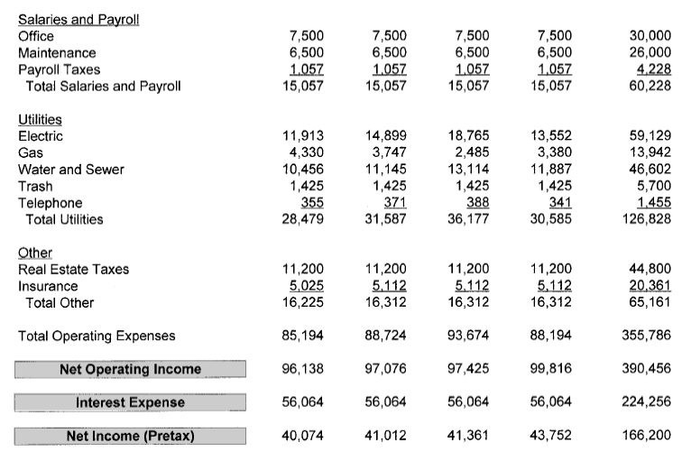
Take a moment to study Table 9.1 to better understand how the various components of an income statement work together. The income statement presented in this example is designed to serve an investor in the rental business and would be used primarily for a multifamily property. It can easily be modified by eliminating categories that are not needed or by adding additional categories to suit the needs of the individual business or entity. For example, the owner of a commercial building would not need all of the items shown in this example. Many of the expenses, such as common area maintenance and taxes, are passed directly through to the ten- ants. The income statement can easily be modified to reflect the specific needs of the company it serves. Investors who take the time to study and review the income statements of many properties will soon be able to understand their informational content and make sound buy-and-sell decisions based on the information presented in them.

 

 

 

 

 

 

 

 

 

 

 

 

 

 

 

 

 

 

 

 

 

 

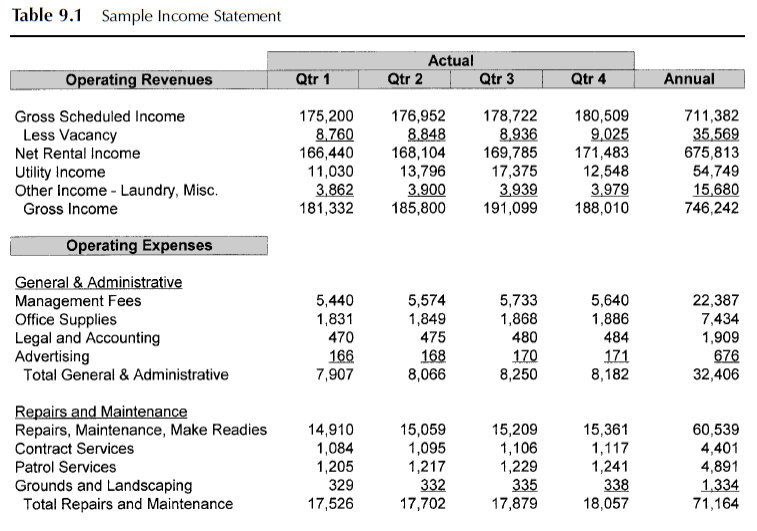
The first primary category on the income statement is operating revenues. Operating revenues for rental property consist of all sources of revenue such as gross scheduled income, vacancy loss, utility income, and other income. Gross scheduled income represents 100 percent of the potential income of a rental property if every single unit or space were occupied. In other words, if the vacancy rate were zero and every tenant paid 100 percent of their respective rent, the rental income for the property would be maximized. Vacancy loss represents the amount of income lost due to the unrented units. Promotional discounts and concessions, as well as delinquencies, also fall under the vacancy loss category. Other income includes income collected for late fees, application fees, laundry room income, vending machine income, and any income that may be collected for utilities. It can also include income for interest earned on money held in interest-bearing accounts such as money market accounts.

 

The second primary category on the income statement is operating expenses. This includes all of the expenses having to do with actually operating an income-producing property, such as general and administrative, payroll, repairs and maintenance, utilities, and taxes and insurance. It does not include depreciation expense, interest expense, or any debt service. Depreciation is, of course, expensed for tax purposes, but that is treated separately on a statement prepared explicitly for federal tax purposes. The purpose in this section is to better understand the income statement so that it can be used to evaluate a property for its value using the income capitalization method, and also to enable us to better forecast the property’s potential for future earnings. Since depreciation is not a true expense in the sense that it affects the cash account (except for smaller capital improvements), it is not usually included on a standard income statement for financial reporting purposes. Since we are not concerned with the tax consequences at this juncture, we will disregard depreciation.

 

General and administrative expenses include disbursements for items such as office supplies, legal and accounting fees, advertising and marketing expenses, and property management fees. Payroll expenses would consist of all expenses related to those personnel directly employed by the entity operating the rental property. Related expenses include payroll for office personnel, maintenance and grounds employees, payroll taxes, workers’ compensation, state and federal employee taxes, and benefits such as insurance and

401(k) programs. Payroll expenses should not include any costs for work performed by subcontractors, even though you may furnish all of the materials and pay the subcontractors only for their labor. These types of expenses fall under repairs and maintenance. Make- readies for apartments, contract services, security and patrol services, general repairs and related materials, and landscaping services should all be included in repairs and maintenance. Utility expenses consist of all disbursements related to a rental property’s utility usage, such as electric, gas, water and sewer, trash removal, cable services, and telephone expenditures. In many instances, these costs are passed on directly to the tenants and would therefore not be included here.

 

Taxes and insurance expense also fall into the operating expenses category. They typically include disbursements for real estate taxes and insurance premiums for physical assets such as the building and any loss of income resulting from damage to the premises. Insurance premiums for boiler equipment, pumps, swimming pool equip- ment, and other machinery also fall into this category. Depending on the specific type of property being operated, many of these subcategories may or may not be required. In addition, there may also be some missing for your particular purposes. This section is provided to give investors a general idea of items that can be found on an income statement and is not intended to be all-inclusive.

The third primary category on the income statement is net operating income (NOI). Although NOI is generally just a single line item, this is the most important element of an income statement. Net operating income is calculated as follows:

 

Gross income − total operating expenses = net operating income

 

Net operating income is the income remaining after all operating expenses have been accounted for. It is also the amount of income available to service any of the property’s related debt. In addition, net operating income is the numerator in the quotient used to calculate the capitalization rate, or cap rate, which was discussed in detail in Chapter 8 under the “Income Capitalization Method” of valuing income-producing properties.

 

The fourth primary category on the income statement is interest expense. This category includes the interest portion of any debt payments being made on the property. Interest expense is placed below net operating income rather than above it in operating expenses since the method in which a particular piece of investment property is funded and capitalized varies widely. For example, Investor A might purchase a commercial strip center using 85 percent debt and only 15 percent equity, while Investor B may choose to purchase an identical building using 50 percent debt and 50 percent equity. If interest expense were treated under the operating expense category, the resulting net operating income for both properties would be different. This is because Investor A’s interest expense is higher because he is using 85 percent debt. Meanwhile, Investor B’s interest expense would be lower because she is using a financing structure comprised of only 50 percent debt. If Investor C wanted to purchase one of the two buildings for her own investment portfolio, she would not be able to evaluate them consistently, because the financing structures are different. It would appear to Investor C that Investor B’s retail strip center was more profitable than Investor A’s property, because Investor B has a lower interest expense.

 

If this seems a little confusing, review the income statement shown in Table 9.1 and experiment with interest expense by moving it above the NOI category. Recall also that net operating income is the numerator in the quotient used to calculate the cap rate. Since NOI would be different for Investor A’s property and Investor B’s property, either the resulting cap rate would be different or the property value itself would have to be different to achieve the same cap rate.

 

The fifth primary category on the income statement is net income. Net income is simply the difference between net operating income and interest expense. In the example in Table 9.1, the figure shown is pretax net income and not after-tax net income. External users of financial statements are not necessarily concerned with how much tax the owner or seller of a property is paying because their tax rate is likely to be different. After-tax net income would very likely be different from owner to owner for smaller to midsized properties.

 

BALANCE STATEMENT

 

The second financial statement most commonly used by investors is the balance statement, or balance sheet as it is sometimes referred to, which is used to report a property’s assets, liabilities, and equity. It reports a property’s financial position at a specific point in time. In effect, the balance statement provides both internal and external users with a snapshot of an income-producing property’s financial position on a specific date. Reports are most often printed at monthly, quarterly, and annual intervals. The balance statement can be useful in providing information about a property’s liquidity and its financial flexibility, which can be critical at times to meet unexpected short- term obligations. An external user such as a lender, for example, may examine the debt-to-equity ratio and determine that the business is already highly leveraged and that no remaining borrowing capacity exists.

 

The balance sheet can also be used in measuring the profitability of an income-producing property. For example, by relating a company’s net income to the owner’s equity or to the total assets, returns can be calculated and used to assess the company’s level of profitability relative to similar businesses.

The return on assets (ROA) is used to measure the relationship between net income and total assets. In other words, the ratio measures the return on the total assets deployed by a business. It is calculated as follows:

 

                     net income

Return on assets =     ——        =  ROA

                    total assets

 

                   $166,200

ROA =                —— = 4.46%

                  $3,727,060

 

 

 

The Return On Equity, or ROE, is used to measure the relation- ship between Net Income and Total Capital. This ratio helps mea- sure the return on an investor’s total equity in a property. It is calculated as follows:

 

                       net income

Return on equity =         —— = ROE

                      total capital

 

                      $166,200

ROE =                     — = 25.38%

                      $654,764

 

 

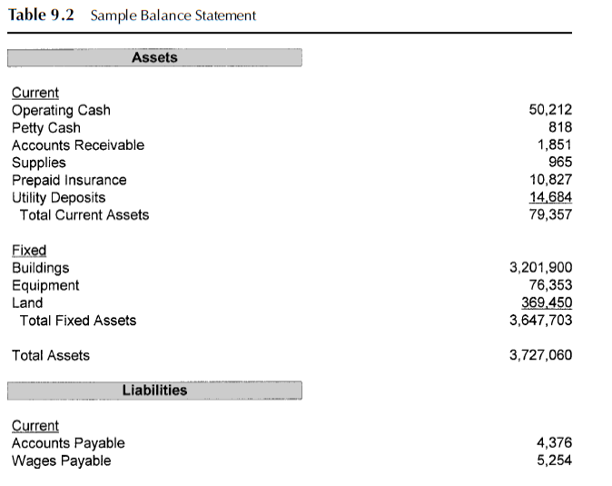
Now take a look at Table 9.2 to better understand how the various components of a balance statement work together. The balance statement illustrated in this example is designed to serve an investor in the rental business and could be used for owners of single-family, multifamily, or commercial properties. The statement can easily be modified by eliminating those categories that are not needed or by adding additional categories to suit the needs of the individual business or entity.

Three primary categories are part of every balance statement: assets, liabilities, and equity. Take a moment to review the following balance sheet equations.

 

Assets = liabilities + equity

Assets − liabilities = equity

Assets − equity = liabilities

Observe that the two sides of the equation are equal, hence the name balance statement. The two sides of the balance sheet must always equal each other, since one side shows the resources of the business and the other side shows who furnished the resources (i.e., the creditors). The difference between the two is the equity.

 

The first primary category on a balance statement is known as a company’s assets. The assets of a business are the properties or economic resources owned by the business and are typically classified as either current or noncurrent assets. Current assets are those that are expected to be converted into cash or used or consumed within a relatively short period of time, generally within a one-year operating cycle. Noncurrent, or fixed assets, are those assets whose benefits extend over periods longer than the one-year operating cycle. For income-producing properties, current assets include amounts owed but not yet collected, such as accounts receivable, cash, security deposits (with utility companies or suppliers, for example), prepaid items such as insurance premiums, and supplies. Fixed assets include items such as buildings, equipment, and land.

 

The second primary category on a balance statement is known as a company’s liabilities. The liabilities of a business are its debts, or any claim another business or individual may have against the operating entity. Liabilities can also be classified as current or noncurrent. Current liabilities are those that will require the use of current assets or that will be discharged within a relatively short period of time, usually within one year. Noncurrent, or long-term liabilities, are those liabilities longer than one year in duration. Current liabilities include amounts owed to creditors for goods and services purchased on credit, such as accounts payable, salaries and wages owed to employees or contractors, security deposits (deposits made by the tenants prior to moving in), taxes payable, and notes payable. Long- term liabilities include mortgages payable and any kind of secondary financing secured against the property, such as loans for capital improvements or equipment financing.

 

The third primary category on a balance statement is known as a company’s equity. The equity of a business represents that portion of value remaining after all obligations have been satisfied. In other words, if an investor’s position in an entity were to be completely liquidated by selling off all of the assets and subsequently satisfying all of the creditors, any remaining proceeds would represent the equity. Since the law gives creditors the right to force the sale of the assets of the business to meet their claims, the equity in a business is considered to be subordinate to the debt. In the event a company declares bankruptcy, obligations to the creditors are satisfied first, and obligations to owners or shareholders are satisfied last.

 

 

 

 

 

 

 

 

 

 

 

 

 

 

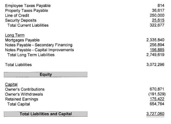
The two primary categories of equity are (1) owner’s contributions and (2) retained earnings. The owner’s equity represents that portion of capital that an investor has personally invested. For example, if an investor put down $400,000 on a $2.5 million commercial building and later spent an additional $150,000 in capital improvements, the owner’s equity would be $550,000. Retained earnings represent that portion of income left in or retained by the business. If a business generates positive earnings, those earnings are referred to as net income and consequently increase the retained earnings account. Conversely, if a business generates negative earnings, those earnings are referred to as a net loss and consequently decrease the retained earnings account. If the company has positive earnings, and those earnings are not left in the company but are instead paid out to the owner, then the equity decreases by a corresponding amount as a result of the owner’s draw.

 

STATEMENT OF CASH FLOWS

 

The third financial statement most commonly used by investors is the statement of cash flows, which is used to measure the cash inflows and outflows produced by the various operating, investing, and financing activities of a business. These activities affect companies and their respective financial statements in different ways. For example, income may flow into an investor’s apartment building from its rental operations and subsequently flow out of it through the purchase of new equipment. In this example, both the income statement and the balance statement are affected, since cash flows in from rents and is then disbursed to purchase assets such as equipment.

 

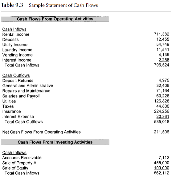
Whereas the balance statement measures a firm’s assets, liabilities, and equity at a specific point in time, the statement of cash flows measures a firm’s operating, investing, and financing activities over a period of time. It can be used to measure cash flows over a month, a quarter, or an entire year. The statement of cash flows is intended to be used in conjunction with both the income statement and the balance statement. By using all three financial statements together, both internal and external users can better evaluate the strengths and weaknesses of a company. Take a moment to review the statement of cash flows in Table 9.3.

 

Cash flow activities are commonly categorized as either operating, investing, or financing activities. Cash inflows from operating activities as they pertain to income-producing properties include income collected from rents, deposits, utility income, laundry and vending income, and interest income. Essentially, any source of cash that flows through the income statement under the heading of operating revenues qualifies as a cash inflow from operating activities. Cash outflows from operating activities includes expenditures made, such as those for management, repairs and maintenance, landscaping, property taxes, insurance, and payments to suppliers. Essentially, any source of cash that flows out of the business under the heading of operating expenses qualifies as a cash outflow from operating activities.

Cash inflows from investing activities as they pertain to income- producing properties include the sale of assets, collections on loans or credit that have been extended (e.g., accounts receivable), and the sale of debt or equity instruments. A real estate investment company that holds several properties in its portfolio may, for example, sell one of its buildings. Doing so would be classified as a cash inflow from investing activities, since one of the assets, a building, was sold. Cash outflows from investing activities include the purchase of assets, the extension of credit or loans, and the purchase of debt or equity instruments. A real estate investment company, for instance, may decide to diversify by investing its excess cash in the securities of another company in an unrelated industry. Doing so would be classified as a cash outflow from investing activities, since an asset such as securities were purchased.

 

Cash inflows from financing activities as they pertain to income- producing properties include the issuance of long-term debt or equity securities, as well as funds obtained through any type of borrowing activity. For example, a real estate investment company may obtain a mortgage to purchase an office building to add to its portfolio of properties, or it may secure a line of credit to make capital improvements. Cash outflows from financing activities include the payment of dividends on equity issued, repurchasing debt or equity that had been issued, and the repayment of borrowed funds. A real estate investment company may, for example, decide to repurchase a series of bonds that were issued to raise cash. Doing so would be classified as a cash outflow from financing activities.

 

 

 

 

 

 

 

 

 

 

 

 

 

 

 

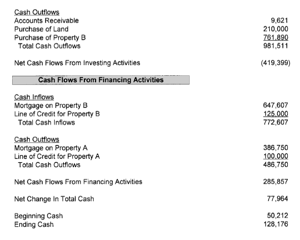
Finally, the net changes in cash flow from operating, investing, and financing activities are aggregated to provide the total change in cash flows for a company. To reconcile the statement of cash flows, the cash at the beginning of the period is added to the net change in total cash, which should match the cash at the end of the period. For example, in Table 9.3, assume the period measured was from the beginning of the calendar year, or January 1, to the end of the calendar year, or December 31. The beginning cash on January 1 is $50,212. That figure is then added to the net change in total cash of $77,964 to provide the ending cash of $128,176. This amount should match exactly the amount of cash shown on the balance statement on December 31.

 

In summary, the income statement, balance statement, and statement of cash flows provide both internal and external users with vital information about the financial well-being of a company or business. They are equally as useful to investors evaluating potential income- producing properties. The balance statement is a static instrument that reflects a company’s financial position at a specific point in time. The income statement and statement of cash flows, on the other hand, are dynamic instruments that reflect a company’s financial position, and changes in its position, over a period of time Using these financial statements in conjunction with each other will provide the most benefit to investors evaluating potential investment opportunities

 

In this example, three comparable sales of properties similar in characteristics and close in size to the subject property were used. The objective was to use houses in desirable locations also having lake views. In the subject property section, simply enter in the purchase price of the house being analyzed. In this example, the original asking price by the seller was $370,000. The asking price is a good place to begin the analysis, but users can also easily experiment with the model by merely changing the asking price, which is exactly what we are going to do in Table 10.2. After entering the purchase price, the square footage of the subject property is entered, which in this example is 2,800. The average sales price per square foot from the comps section is then fed into the subject property section. The purchase price per square foot is automatically calculated and then multiplied by the square footage of the subject property under the property values and adjustment to comps sections.

 

The adjustment to comps cell is used to create an estimated fair market value (FMV) using a range of property values for three different scenarios—best case, most likely, and worst case. In this case study, $2.50 per square foot is used; however, the number can be changed to anything you want it to be. For the best-case estimated fair market value, the model adds $2.50 to the price per square foot cell in the comp averages section, and then multiplies the sum of the two by the square feet of the subject property. The positive value of $2.50 is visible under the adjustment to comps heading. Here’s how the calculation works:

 

 

Best-Case Estimate of Fair Market Value

 

(Average price per square foot + adjustment to comps)

 

× subject property square feet = best-case estimate of FMV ($137.127 + $2.50) × 2,800 = $390,956

 

 

The most likely estimate of the FMV calculation in the model neither adds nor subtracts the value of $2.50 to the price per square foot cell in the comp averages section. As you can see in Table 10.1, it is set to zero. This calculation is merely the product of the average price per square foot and the number of square feet. Take a moment to examine the calculation.

 

Most Likely Estimate of Fair Market Value

 

Average price per square foot × subject property square feet

 

= most likely estimate of FMV $137.127 × 2,800 = $383,956

 

For the worst-case estimate of FMV, the model subtracts $2.50 from the price per square foot cell in the comp averages section, and then multiplies the difference of the two by the number of square feet of the subject property. Take a minute to review the calculations.

 

Worst-Case Estimate of Fair Market Value

 

(Average price per square foot − adjustment to comps)

 

× subject property square feet = worst-case estimate of FMV ($137.127 − $2.50) × 2,800 = $376,956

 

The purpose of creating three different scenarios in the model is to provide a range of estimated fair market values. This allows the user to evaluate the very minimum FMV that might be expected on the low end of the price range, and the very highest FMV that might be expected on the high end of the price range. In this example, using $2.50 provides a total range of $5.00 per square foot—from +$2.50 to −$2.50.

 

Now let’s take a moment to interpret the output. What is the model telling us? The three different values provide us with a minimum estimate for FMV and a range of values up to a maximum estimate for FMV. In order for the subject property to pass the first of the two tests, which is the comparable sales test, it must meet a minimum threshold of any value greater than zero by taking the difference of the FMV and the actual purchase price. In this example, the subject property passes the test under all three price scenarios reflected in the model, with positive values of $20,956 for the best-case estimate, $13,956 for the most likely estimate, and $6,956 for the worst-case estimate. If everything else looks good in the rest of the model, it is acceptable to have a negative value under the worst-case estimate. The most likely and best-case estimates, however, must have positive values. The difference in values shown in each of these three scenarios represents a discount of the actual purchase price to the market. So far, so good. Our subject property has passed the first test.

 

Scenario I

 

 

 

Scenario II

 

 

 

Scenario III

 

 

 

If you don't start pulling your weight around here its going to be shape up, or... ship up.

Hola, is Rosa still alive? No? Well this is not my day. Look at us, crying like a couple of girls on the last day of camp. Great, now I'm gonna smell to high heaven like a tuna melt! Te quiero. English, please. I love you! Great, now I'm late. Perhaps an attic shall I seek.

Hola, is Rosa still alive? No? Well this is not my day. Look at us, crying like a couple of girls on the last day of camp. Great, now I'm gonna smell to high heaven like a tuna melt! Te quiero. English, please. I love you! Great, now I'm late. Perhaps an attic shall I seek.